Getting started#
If you have installed the packed with pip then you should have a command called cardiac-geometries available. The cardiac-geometries package comes with a a few useful cli commands and you can list information about these commands using
cardiac-geometries --help
At the time of writing (version 0.3.1), the output look as follows
$ cardiac-geometries --help

 Usage: cardiac-geometries [OPTIONS] COMMAND [ARGS]...

 Cardiac Geometries - A library for creating meshes of cardiac geometries

╭─ Options ─────────────────────────────────────────────────────────────────────────────╮
│ --version      Show the version and exit.                                             │
│ --help         Show this message and exit.                                            │
╰───────────────────────────────────────────────────────────────────────────────────────╯
╭─ Commands ────────────────────────────────────────────────────────────────────────────╮
│ create-lv-ellipsoid                                                                   │
│ create-slab                                                                           │
│ fibers-to-xdmf       Convert microstructure.h5 into separate .xdmf-files for f0, s0,  │
│                      and n0. Assumes a folder containing a 'mesh.xdmf' and            │
│                      'microstructure.h5'.                                             │
│ folder2h5            Convert folder with geometry files to a single file              │
╰───────────────────────────────────────────────────────────────────────────────────────╯
To see more information about the individual subcommands you can use the --help flag on the subcommand, e.g cardiac geometries create-slab --help.
Run using docker#
cardiac-geometries depends on both FEniCS and gmsh which might be challenging to install. Therefore we provide a docker image at
ghcr.io/computationalphysiology/cardiac_geometries:latest
To run the cardiac-geometries help command you can use the following command
docker run --rm -v $PWD:/home/shared -w /home/shared -t ghcr.io/computationalphysiology/cardiac_geometries:latest cardiac-geometries --help
This will also mount your current directory into the working directory of the container so that you have access to your current directory within the docker container.
Creating a slab#
You can create a slab geometry (i.e a box mesh) by using the following command
cardiac-geometries create-slab slab
This will create a new directory slab with the following content
slab
├── ffun.h5
├── ffun.xdmf
├── info.json
├── markers.json
├── mesh.h5
├── mesh.xdmf
├── slab.h5
├── slab.json
├── slab.msh
├── triangle_mesh.h5
└── triangle_mesh.xdmf
Here the .msh file that is created by gmsh and contains the mesh with all the physical surfaces.
The .xmdf files are files that you can open in paraview to inspect the geometry.
mesh.xdmf contains the mesh and the volumetric subdomains, triangle_mesh.xdmf contains the facet subdomains and your might also see line_mesh.xdmf and vertex_mesh.xdmf which contains the subdomains for the edges and vertices. You will also see a ffun.xdmf which contains a FEniCS facet function. This is similar to triangle_mesh.xdmf however ffun.xdmf also contains information about the mesh to that you can load the facet function directly without going via a MeshValueCollection.
The file markers.json contains a dictionary to the markers for the different subdomains. For the slab, the default markers are
{"X0": [1, 2], "X1": [2, 2], "Y0": [3, 2], "Y1": [4, 2], "Z0": [5, 2], "Z1": [6, 2], "Myocardium": [7, 3]}
Each value has two numbers where the first number represents the marker and the second the dimension. For example X0 has the marker 1 for dimension 2 (i.e facets), and are the markers for the \(x=0\) plane. X1 is the marker for the \(x=l_x\) plane. In the script you can specify the length in the \(x, y\) and \(z\) direction through the arguments lx, ly and lz respectively. In this case the domain will be the box \([0, l_x] \times [0, l_y] \times [0, l_z]\) where is assumed that the apex is located at the place \(z = 0\), the base at \(z = l_z\), the endocardium at \(y = 0\) and the epicardium at \(y = l_y\). Also here you can generate fibers with the same rule based approach.
The file info.json contains parameters used to create the mesh as well as a timestamp and the version of cardiac-geometries used to create the mesh.
The file slab.h5 contains all the data collected in one single file. This is useful if you want to use the geometry in a simulation for example. The file slab.json contains the schema used for the file and is used when loading the data. This might be relevant if you want to save data in another format. The schema is discussed in more detailed further down in this document.
Schema#
Every object is represented as an entry in the schema (i.e in the file called slab.json in the slab example). Each entry contains a set of key value pairs where the keys are the same for every object but the values might be different. For example the mesh object has the following key-value pairs
"mesh": {
    "h5group": "/mesh",
    "fname": "mesh.xdmf",
    "mesh_key": "",
    "is_dolfin": true,
    "is_mesh": true,
    "is_meshfunction": false,
    "is_function": false,
    "dim": -1
  },
Here h5group would by the location of the mesh inside the file containing all the data (i.e slab.h5). This means that if you wanted to load this mesh in FEniCS you could do
import dolfin

mesh = dolfin.Mesh()
with dolfin.HDF5File(mesh.mpi_comm(), "slab.h5", "r") as h5file:
    h5file.read(mesh, "/mesh", True)
(where the third argument is a boolean value indicating that we should use the partition from the file).
fname would be the corresponding single file generated by the script which is a file you can open in paraview. mesh_key would indicate the key to the mesh used by the object. Since this is a mesh itself, it does not apply and the value is therefore empty. is_dolfin indicated that this is a FEniCS object and to read it you need to use dolfin.HDF5File. If is_dolfin is false then you should use h5py instead. You can read more about how to load the data further down in this document.
is_mesh, is_meshfunction and is_function are just boolean values where only one can be true (it is also possible that all are false in which case is_dolfin is also false). In this case we have a mesh and therefore is_mesh is true. Finally dim is a value that is used for the meshfunctions to indicate which dimension the meshfunction covers. In this case the value is set to -1 which means that this value is not used.
Let us look at the example with the face function ffun which has the following entry in the schema
"ffun": {
    "h5group": "/meshfunctions/ffun",
    "fname": "triangle_mesh.xdmf:name_to_read",
    "mesh_key": "mesh",
    "is_dolfin": true,
    "is_mesh": false,
    "is_meshfunction": true,
    "is_function": false,
    "dim": 2
  },
First thing you should note is that the mesh_key is set to mesh which is the key of the mesh that we first looked that. Since this is also a meshfunction and the dimension is 2 we know that the object should be constructed as follows
ffun = dolfin.MeshFunction("size_t", mesh, 2)
Another thing to note is that the fname both contains a filename (i.e triangle_mesh.xdmf) and a group (i.e name_to_read). This only means that the values are located in a group called named_to_read in the XDMF-file (this is just the default name in gmsh).
The entry for info has a little bit different values
  "info": {
    "h5group": "/info",
    "fname": "info.json",
    "mesh_key": "",
    "is_dolfin": false,
    "is_mesh": false,
    "is_meshfunction": false,
    "is_function": false,
    "dim": -1
  },
First of all, this is not a dolfin object so is_dolfin is set to false.
Generating microstructure#
It is also possible to create microstructure vector fields (i.e fibers, sheets and cross sheets). You can use this by passing the flag --create-fibers.
For the slab this will use a fiber angle on the endocardium (i.e \(y = 0\)), which you can specify with the flag --fiber-angle-endo, and another angle on the epicardium (\(y = l_y\)), which you can specify with the flag --fiber-angle-epi, and make a linear transition between the two planes. One example is shown below with fiber-angle-endo=-60 and fiber-angle-epi=60
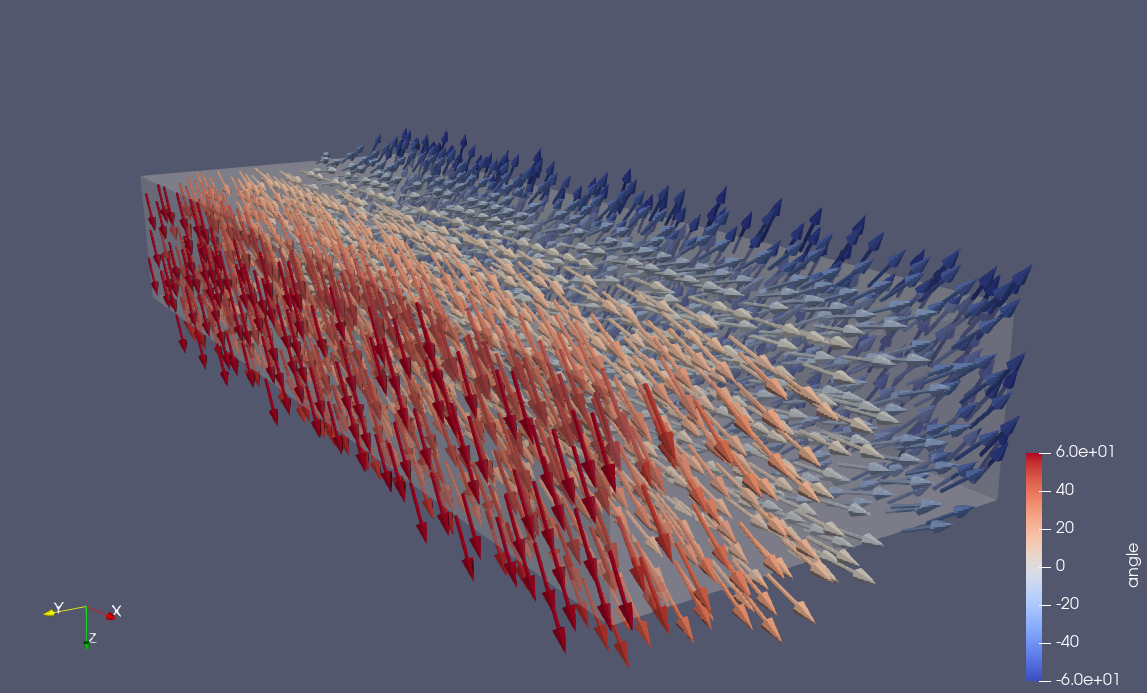
Fig. 1 Fibers on the slab with \(-60^{\circ}\) angle on the endocardium and \(60^{\circ}\) angle on the epicardium.#
When running with the --create-fibers flag you will also see another file appearing the folder called microstructure.h5 that contains the fibers, sheets and cross sheet vector fields. To visualize these in Paraview you need to first run the fibers-to-xdmf command and pass in the folder.
Notice also that the schema now has entries for the microstructure, for example the entry
"f0": {
    "h5group": "/microstructure/f0",
    "fname": "microstructure.h5:f0",
    "mesh_key": "mesh",
    "is_dolfin": true,
    "is_mesh": false,
    "is_meshfunction": false,
    "is_function": true,
    "dim": -1
  },
is the entry for the fibers and we can see that this entry has is_function set to true.
Loading the data#
In cardiac-geometries there is also a way to load the data into python using the Geometry class located in the module cardiac_geometries.geometry.
We can load the slab data as follows
from cardiac_geometries.geometry import Geometry

geo = Geometry.from_file("slab/slab.h5", schema_path="slab/slab.json")
This object will now contain the objects listed in the schema and if there is an entry listed in the schema that is not contained in the file it will throw a RuntimeError.
Saving the data in another format#
One way to use the Geometry class is to load data using one schema and save it with another. Say for example that you want to combine two meshes into one file, then you can for example to the following
from cardiac_geometries.geometry import Geometry

geo1 = Geometry.from_file("slab1/slab.h5", schema_path="slab1/slab.json")
geo2 = Geometry.from_file("slab2/slab.h5", schema_path="slab2/slab.json")

scheme = {
        "info1": H5Path(h5group="geo1/info", is_dolfin=False),
        "mesh1": H5Path(h5group="geo1/mesh", is_mesh=True),
        "info2": H5Path(h5group="geo2/info", is_dolfin=False),
        "mesh2": H5Path(h5group="geo2/mesh", is_mesh=True),
}

geo = Geometry(
    mesh1=geo1.mesh, info1=geo1.info,
    mesh2=geo2.mesh, info2=geo2.info,
    scheme=scheme
)
# This will also create a file double_slab.json with the scheme
geo.save("double_slab.h5")
Creating a slab in a bath#
In many applications of cardiac electrophysiology it is common to study the bath-loading effects, see e.g
Bishop, Martin J., and Gernot Plank. “Representing cardiac bidomain bath-loading effects by an augmented monodomain approach: application to complex ventricular models.” IEEE Transactions on Biomedical Engineering 58.4 (2011): 1066-1075.
In this case it is of interest to create a slab surrounded by a conducting media. This can be done with the following command
cardiac-geometries create-slab-in-bath slab_in_bath --lx=1.0 --ly=2.0 --ly=3.0 --bx=0.1 --by=0.2 --bz=0.3 --dx=0.05
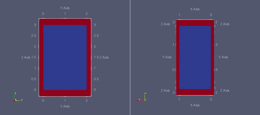
Fig. 2 Slab geometry of dimension \([0, l_x] \times [0, ly] \times [0, lz] = [0, 1] \times [0, 2] \times [0, 2]\) embedded in a bath of width \(b_x = 0.1\), \(b_y = 0.2\) and \(b_z = 0.3\) respectively in the \(x-, y-\) and \(z\) direction.#
Creating a lv ellipsoid#
You can create a left ellipsoidal ventricular geometry by using the following command
cardiac-geometries create-lv-ellipsoid lv-mesh
Similar to the slab it can also create analytic fiber orientations.
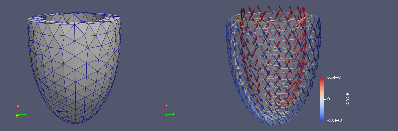
Fig. 3 LV-ellipsoidal mesh and fibers with \(-60^{\circ}\) angle on the endocardium and \(60^{\circ}\) angle on the epicardium.#
Creating the mesh from the Land Cardiac Mechanics Benchmark paper#
Land S, Gurev V, Arens S, Augustin CM, Baron L, Blake R, Bradley C, Castro S, Crozier A, Favino M, Fastl TE. Verification of cardiac mechanics software: benchmark problems and solutions for testing active and passive material behaviour. Proc. R. Soc. A. 2015 Dec 8;471(2184):20150641.
To create the geometry from the Land Cardiac Mechanics Benchmark paper you can use the following command
cardiac-geometries create-lv-ellipsoid benchmark-mesh --create-fibers --r-short-endo=7 --r-short-epi=10 --r-long-endo=17 --r-long-epi=20 --mu-apex-endo=0 --mu-apex-epi=0 --mu-base-endo=1.869328527979773 --mu-base-epi=1.8234765819369754 --psize-ref=3
Note that this mesh will have a flat base located at \(z_{\text{base}} = 5\). The mu-base-endo and mu-base-epi is computed using the following formula
and
which means that if you want the base to be located at \(z = 0\) you can set \(\mu_{\text{base}}^{\text{endo}} = \mu_{\text{base}}^{\text{epi}} = \frac{\pi}{2} \approx 1.5707963267948966\), i.e
cardiac-geometries create-lv-ellipsoid mymesh --create-fibers --r-short-endo=7 --r-short-epi=10 --r-long-endo=17 --r-long-epi=20 --mu-apex-endo=0 --mu-apex-epi=0 --mu-base-endo=1.5707963267948966 --mu-base-epi=1.5707963267948966 --psize-ref=3
Creating a BiV ellipsoid#
There is also an option to create BiV ellipsoid using the create-biv-ellipsoid command, e.g
cardiac-geometries create-biv-ellipsoid biv --char-length 0.1 --create-fibers
will create the following mesh with fibers. Note that the fibers are not analytically computed, and you are therefore required to install ldrb if you want to create fibers.
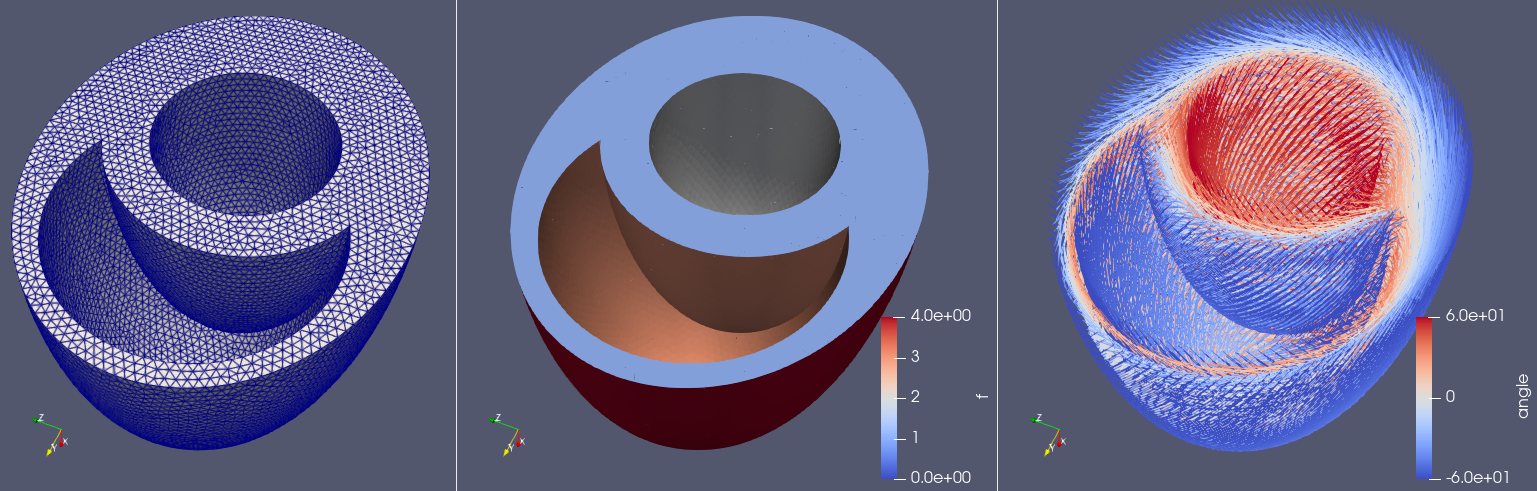
Fig. 4 BiV-ellipsoidal mesh, facet markers and fibers with \(-60^{\circ}\) angle on the endocardium and \(60^{\circ}\) angle on the epicardium.#
Creating a BiV ellipsoid embedded in a torso#
It is also possible to take the same idealized BiV geometry and embed it in an idealized torso (i.e a BoX) using the command create-biv-ellipsoid-torso, e.g
cardiac-geometries create-biv-ellipsoid-torso biv_torso --char-length 0.7 --torso-length 30 --torso-width 30 --torso-height 30 --rotation-angle 0.4
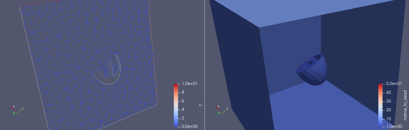
Fig. 5 Idealized BiV embedded in an idealized torso#
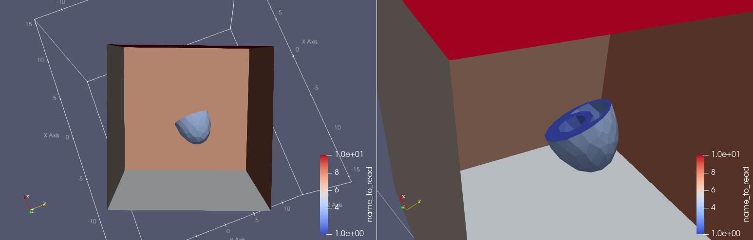
Fig. 6 Showing the facet markers for the biv embedded in a torso#