Content License: Creative Commons Attribution 4.0 International (CC-BY-4.0)

Meshes and microstructure¶

Cylindrical domain¶

We consider a cylindrical domain $\Omega(a, r) = [-a, a] \times \omega(r)$ with

\omega(r) = \{ (y, z) \in \mathbb{R}^2 : y^2 + z^2 < r \}

(1)

We let $a = 2000 \mu m$ and $r = 300 \mu m$ and will refer to $\Omega_0$ as $\Omega(300, 2000)$

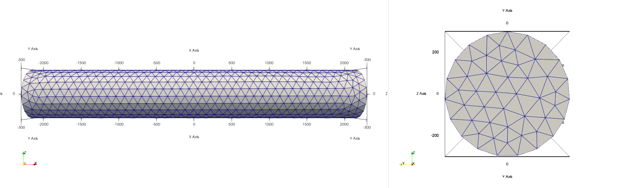
Cylindrical domain — Figure 1:Cylindrical mesh with $a = 2000 \mu m$ and $r = 300 \mu m$

For the cylinder we also define a local coordinate system in the longitudinal (aka fiber) direction

In our case we orient the fibers along the height the cylinder, i.e

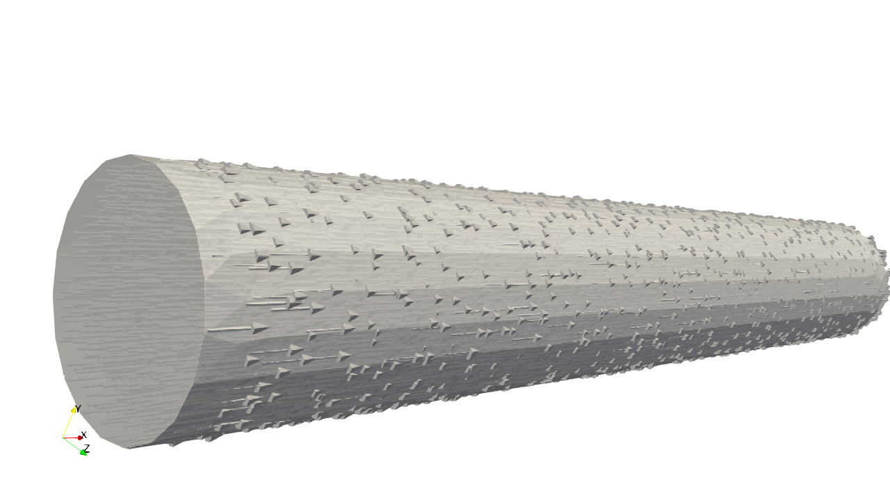
\mathbf{f}_0 = \begin{pmatrix} 1 \\ 0 \\ 0 \end{pmatrix}

(2)

Figure 2:Showing the orientation of the cardiac fibers for the cylinder along the longitudinal direction

In a cylinder there is a natural decomposition into radial and circumferential components. We have the radial basis function given by

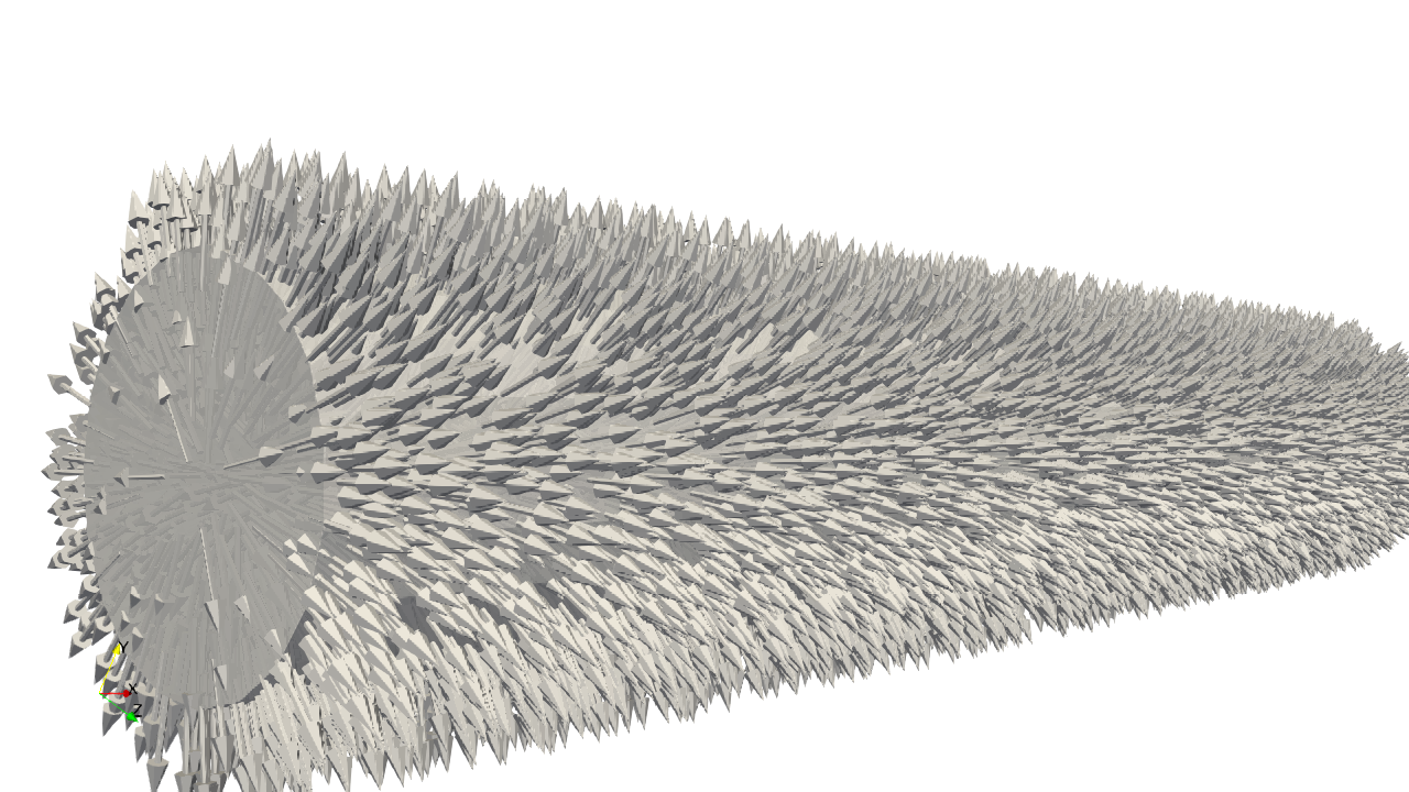
\mathbf{e}_r = \begin{pmatrix} 0 \\ y / (y^2 + z^2) \\ z / (y^2 + z^2) \end{pmatrix}

(3)

Radial — Figure 3:Showing the orientation of radial components

and the circumferential basis function given by

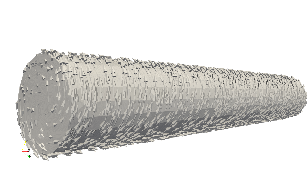
\mathbf{e}_c = \begin{pmatrix} 0 \\ z / (y^2 + z^2) \\ -y / (y^2 + z^2) \end{pmatrix}

(4)

Circ — Figure 4:Showing the orientation of circular components

LV domain¶

We will also test out an idealized LV domain generated using cardiac-geometries

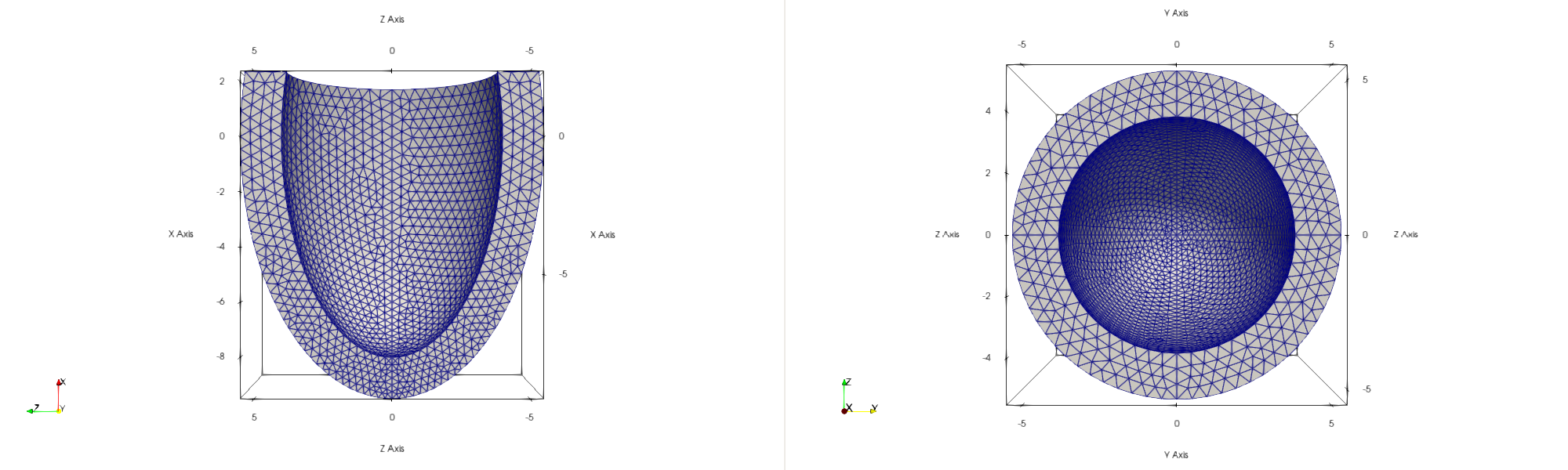
Figure 5:Idealized LV mesh with width of 1.5 mm, a short axis radius of 4 mm and a long axis radius of 8 mm.

For the LV we also have the rule based fiber orientations

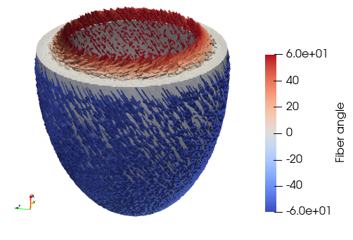
LV fiber — Figure 6:Fiber orientations in the LV with and endo / epi fiber angle of 60/-60.

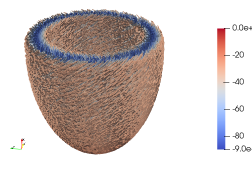
LV sheet — Figure 7:Sheet orientations in the LV.

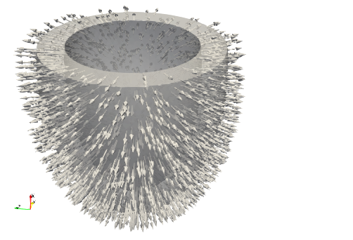
LV sheet normal — Figure 8:Sheet-normal orientations in the LV.

Material model¶

We use the the transversely isotropic version of the Holzapfel Ogden model, i.e

\Psi(\mathbf{F}) = \frac{a}{2 b} \left( e^{ b (I_1 - 3)} -1 \right) + \frac{a_f}{2 b_f} \mathcal{H}(I_{4\mathbf{f}_0} - 1) \left( e^{ b_f (I_{4\mathbf{f}_0} - 1)_+^2} -1 \right) + \kappa (J \mathrm{ln}(J) - J + 1)

(5)

with

(x)_+ = \max\{x,0\}

(6)

and

\mathcal{H}(x) = \begin{cases} 1, & \text{if $x > 0$} \\ 0, & \text{if $x \leq 0$} \end{cases}

(7)

is the Heaviside function. Here

I_1 = \mathrm{tr}(\mathbf{F}^T\mathbf{F})

(8)

and

I_{4\mathbf{f}_0} = (\mathbf{F} \mathbf{f}_0)^T \cdot \mathbf{F} \mathbf{f}_0

(9)

and

J = \mathrm{det}(\mathbf{F})

(10)

with $\mathbf{f}_0$ being the direction the muscle fibers.

Material parameters¶

The material parameter are

Parameter	Value
$a$	2280 Pa
$b$	9.726
$a_f$	1685 Pa
$b_f$	15.779

Modeling of compressibility¶

Modeling of active contraction¶

Similar to Finsberg et. al we use an active strain formulation and decompose the deformation gradient into an active and an elastic part

\mathbf{F} = \mathbf{F}_e \mathbf{F}_a

(11)

with

\mathbf{F}_a = (1 - \gamma) \mathbf{f} \otimes \mathbf{f} + \frac{1}{\sqrt{1 - \gamma}} (\mathbf{I} - \mathbf{f} \otimes \mathbf{f}).

(12)

In these experiments we use $\gamma = 0.2$ to represent end systole.

Variational formulation¶

We model the myocardium as incompressible using a two field variational approach and $\mathbb{P}_2-\mathbb{P}_1$ finite elements for the displacement $\mathbf{u}$ and hydrostatic pressure $p$ . m

The Euler‐Lagrange equations in the Lagrangian form reads: find $(\mathbf{u},p) \in H^1(\Omega_0) \times L^2(\Omega_0)$ such that for all $(\delta \mathbf{u},\delta \mathbf{u}) \in H^1(\Omega_0) \times L^2(\Omega_0)$ we have

\delta \Pi(\mathbf{u}, p) = 0.

(13)

For the cylinder we have

\delta \Pi(\mathbf{u}, p) = \int_{\Omega_0}\left[ \mathbf{P} : \nabla \delta \mathbf{u} - \delta p (J - 1) - pJ \mathbf{F}^{-T}: \delta \mathbf{u} \right] \mathrm{d}V + \int_{\partial \Omega_0^{a} \cup \Omega_0^{-a}} k \mathbf{u} \cdot \delta \mathbf{u} \mathrm{d}S

(14)

where $\Omega_0^{a} = \{ a \} \times \omega(r)$ represents the boundaries at each end of the cylinder. Here we enforce a Robin type boundary condition at both ends of the cylinder with a spring $k$ . This parameter will be used to represent the loading conditions and we choose $k=$ 1 Pa / μm to represent standard loading conditions.

For the left ventricle we have

\delta \Pi(\mathbf{u}, p) = \int_{\Omega_0}\left[ \mathbf{P} : \nabla \delta \mathbf{u} - \delta p (J - 1) - pJ \mathbf{F}^{-T}: \delta \mathbf{u} \right] \mathrm{d}V + \int_{\partial \Omega_0^{\mathrm{epi}}} k \mathbf{u} \cdot \delta \mathbf{u} \mathrm{d}S + \int_{\partial \Omega_0^{\mathrm{endo}}} p_{\mathrm{lv}} J \mathbf{F}^T \mathbf{N} \cdot \delta \mathbf{u} \mathrm{d}S.

(15)

Here we enforce a Robin type boundary condition at the epicardium, $\Omega_0^{\mathrm{epi}}$ , with a spring $k = 0.5$ kPa / mm, and an endocardial pressure $p_{\mathrm{lv}}$ on the endocardium $\Omega_0^{\mathrm{endo}}$ . In addition we fix the basal plane in the longitudinal direction.

Cauchy stress¶

The Cauchy stress tensor is given by

\sigma = J^{-1} \frac{\partial \Psi }{\partial \mathbf{F}} \mathbf{F}^T

(16)

We can extract different components of the Cauchy stress tensor. For example the fiber component can be extracted using the following formula

\sigma_{ff} = \mathbf{f}^T \cdot \sigma \mathbf{f}

(17)

where $\mathbf{f}$ is the vector field displayed in Figure 6 in the current configuration.

Numerical experiments¶

Cylinder¶

For the experiments with the cylinder we simulated two states; one relaxed state and one contracted state. For the contracted state we used $\gamma = 0.2$

Cylinder varying spring¶

We tested different values of the spring constant $k$ , with $k = 3$ Pa / μm, representing standard load, $k = 0.1$ Pa / μm representing unloaded and $k = 10$ kPa / μm representing increased load.

spring Diameter — Figure 9:Resulting diameter at the center for the cylinder in relaxed and contracted state for spring constants

spring Length — Figure 10:Resulting length of the cylinder in relaxed and contracted state for spring constants

spring Strain — Figure 12:Resulting strain the cylinder in the contracted state for different spring constants in the longitudinal $E_{xx}$ , circumferential $E_{c}$ and radial $E_r$ direction

spring Stress — Figure 13:Resulting stress the cylinder in the contracted state for different spring constants in the longitudinal $\sigma_{xx}$ , circumferential $\sigma_{c}$ and radial $\sigma_r$ direction

Twitch¶

To simulate twitch we create a syntetic curve for γ,

\gamma(t) = \begin{cases} \gamma_{\mathrm{min}} & \text{ if } t <= t_0, \\ \frac{\gamma_{\mathrm{max}} - \gamma_{\mathrm{min}}}{\beta} \left( e^{-\frac{t - t_0}{\tau_1}} - e^{-\frac{t - t_0}{\tau_2}} \right) + \gamma_{\mathrm{min}} & \text{ otherwise} \\ \end{cases}

(18)

and

\beta = \left(\frac{\tau_1}{\tau_2}\right)^{- \frac{1}{\frac{\tau_1}{\tau_2} - 1}} - \left(\frac{\tau_1}{\tau_2}\right)^{- \frac{1}{1 - \frac{\tau_2}{\tau_1}}}.

(19)

cylinder_twitch Diameter — Figure 15:Resulting diameter at the center for the cylinder in relaxed and contracted state for spring constants

cylinder_twitch Length — Figure 16:Resulting length of the cylinder in relaxed and contracted state for spring constants

cylinder_twitch Stress — Figure 18:Resulting stress the cylinder in the contracted state for different spring constants in the longitudinal $\sigma_{xx}$ , circumferential $\sigma_{c}$ and radial $\sigma_r$ direction

cylinder_twitch Stress label — Figure 19:Label corresponding to figure Figure 18 showing which regions we average the stress

LV¶

For the LV we have two different states; one where we have no endocardial pressure (referred to as the unloaded state) and one where we apply an endocardial pressure of 15 kPa (referred to as the loaded state). In both cases we set $\gamma = 0.2$ .

LV strain — Figure 20:Strain in the fiber, sheet and sheet normal direction for the unloaded and loaded state

LV stress — Figure 21:Stress in the fiber, sheet and sheet normal direction for the unloaded and loaded state

References¶

Holzapfel, G. A., & Ogden, R. W. (2009). Constitutive modelling of passive myocardium: a structurally based framework for material characterization. Philosophical Transactions of the Royal Society A: Mathematical, Physical and Engineering Sciences, 367(1902), 3445–3475. 10.1098/rsta.2009.0091
Finsberg, H., Xi, C., Tan, J. L., Zhong, L., Genet, M., Sundnes, J., Lee, L. C., & Wall, S. T. (2018). Efficient estimation of personalized biventricular mechanical function employing gradient‐based optimization. International Journal for Numerical Methods in Biomedical Engineering, 34(7). 10.1002/cnm.2982

Material from Ciucci 2024

Simulating mechanical forces