Demo - Fitzhugh-Nagumo neural model

ref: https://en.wikipedia.org/wiki/FitzHugh–Nagumo_model

The FitzHugh–Nagumo model (FHN), named after Richard FitzHugh (1922–2007) who suggested the system in 1961 and J. Nagumo et al. who created the equivalent circuit the following year, describes a prototype of an excitable system (e.g., a neuron).

The FHN Model is an example of a relaxation oscillator because, if the external stimulus \(I_{\text{ext}}\) exceeds a certain threshold value, the system will exhibit a characteristic excursion in phase space, before the variables \(v\) and \(w\) relax back to their rest values.

This behaviour is typical for spike generations (a short, nonlinear elevation of membrane voltage \(v\), diminished over time by a slower, linear recovery variable \(w\)) in a neuron after stimulation by an external input current.

The equations for this dynamical system read

(1)\[\begin{align} \dot{v} &= v - \frac{v^3}{3} -w + RI_{\text{ext}} \\ \tau \dot{w} &= v + a - bw \end{align}\]

The dynamics of this system can be nicely described by zapping between the left and right branch of the cubic nullcline.

The FitzHugh–Nagumo model is a simplified 2D version of the Hodgkin–Huxley model which models in a detailed manner activation and deactivation dynamics of a spiking neuron. In the original papers of FitzHugh, this model was called Bonhoeffer–Van der Pol oscillator (named after Karl-Friedrich Bonhoeffer and Balthasar van der Pol) because it contains the Van der Pol oscillator as a special case for \(a=b=0\). The equivalent circuit was suggested by Jin-ichi Nagumo, Suguru Arimoto, and Shuji Yoshizawa.

Code example

Import the necessary pagages

import ap_features as apf
import matplotlib.pyplot as plt
import numpy as np
from scipy.integrate import solve_ivp

Define the right hand side of the ODE

def fitzhugh_nagumo(t, x, a, b, tau, Iext):
    """Time derivative of the Fitzhugh-Nagumo neural model.
    Parameters

    Parameters
    ----------
    t : float
        Time (not used)
    x : np.ndarray
        State of size 2 - (Membrane potential, Recovery variable)
    a : float
        Parameter in the model
    b : float
        Parameter in the model
    tau : float
        Time scale
    Iext : float
        Constant stimulus current

    Returns
    -------
    np.ndarray
        dx/dt - size 2
    """
    return np.array([x[0] - x[0] ** 3 - x[1] + Iext, (x[0] - a - b * x[1]) / tau])

Select some parameters and solve the system

a = -0.3
b = 1.4
tau = 20
Iext = 0.23
time = np.linspace(0, 999, 1000)
res = solve_ivp(
    fitzhugh_nagumo,
    [0, 1000],
    [0, 0],
    args=(a, b, tau, Iext),
    t_eval=time,
)

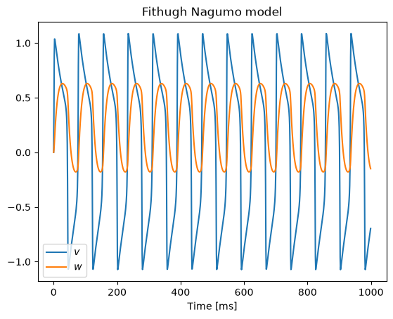
Collect the solutions and create a beats object

v = res.y[0, :]
w = res.y[1, :]

s = apf.Beats(y=v, t=time)

fig, ax = plt.subplots()
ax.plot(time, v, label="$v$")
ax.plot(time, w, label="$w$")
ax.legend()
ax.set_xlabel("Time [ms]")
ax.set_title("Fithugh Nagumo model")
plt.show()

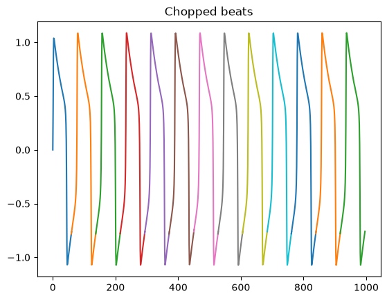
We can now chop the trace into indivisual beats

beats = s.beats
print(beats)

[Beat(t=(61,), y=(61,)), Beat(t=(80,), y=(80,)), Beat(t=(80,), y=(80,)), Beat(t=(80,), y=(80,)), Beat(t=(80,), y=(80,)), Beat(t=(81,), y=(81,)), Beat(t=(79,), y=(79,)), Beat(t=(80,), y=(80,)), Beat(t=(80,), y=(80,)), Beat(t=(79,), y=(79,)), Beat(t=(80,), y=(80,)), Beat(t=(80,), y=(80,)), Beat(t=(80,), y=(80,))]

And plot them

fig, ax = plt.subplots()
for beat in beats:
    ax.plot(beat.t, beat.y)
ax.set_title("Chopped beats")
plt.show()

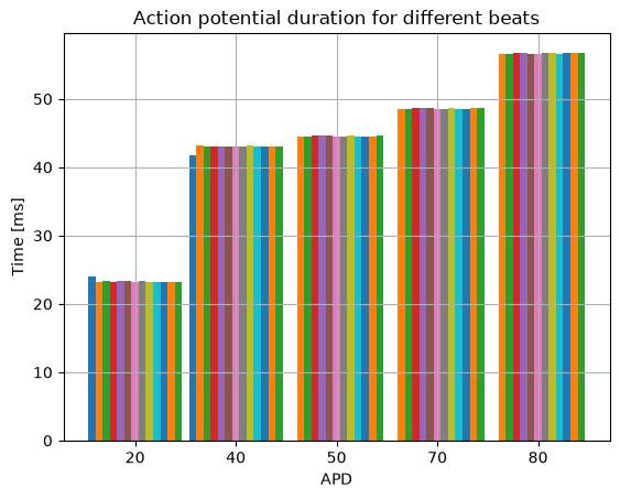
We can also plot the action potential duration for each beat

# Plot some APDs
fig, ax = plt.subplots()
apds = [20, 40, 50, 70, 80]
N = len(apds)
x = np.arange(N)
width = 1 / (s.num_beats + 1)
for i, beat in enumerate(beats):
    ax.bar(x + i * width, [beat.apd(apd) for apd in apds], width=width)
ax.set_xticks(x + 0.5 - width)
ax.set_xticklabels(apds)
ax.set_ylabel("Time [ms]")
ax.set_xlabel("APD")
ax.grid()
ax.set_title("Action potential duration for different beats")
plt.show()

Warning: only one root was found for APD 50

Warning: only one root was found for APD 70

Warning: only one root was found for APD 80