Features#
Here we will go through the different features that we can compute with ap_features.
import matplotlib.pyplot as plt
import numpy as np

import ap_features as apf
Single beat features#
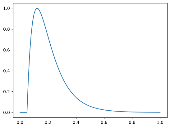
To start with we will go through some features that we can derive from a single beat. To illustrate this we will use a synthetic calcium transient
time = np.linspace(0, 1, 101)
tstart = 0.05
y = apf.testing.ca_transient(t=time, tstart=tstart)

fig, ax = plt.subplots()
ax.plot(time, y)
plt.show()
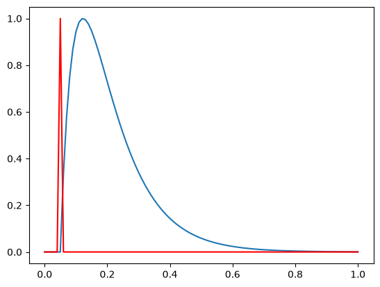
Notice that the trace starts at t=0.05 and we could use a pacing amplitude to indicate this, e.g
pacing = np.zeros_like(time)
pacing[np.isclose(time, tstart)] = 1

fig, ax = plt.subplots()
ax.plot(time, y)
ax.plot(time, pacing, color="red")
plt.show()
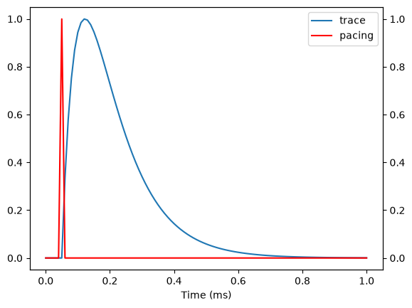
Another way to work with ap_feautres is to convert the trace into a beat, in which case you can do
beat = apf.Beat(y=y, t=time, pacing=pacing)

beat.plot(include_pacing=True)
FigAx(fig=<Figure size 640x480 with 2 Axes>, ax=<Axes: xlabel='Time (ms)'>)
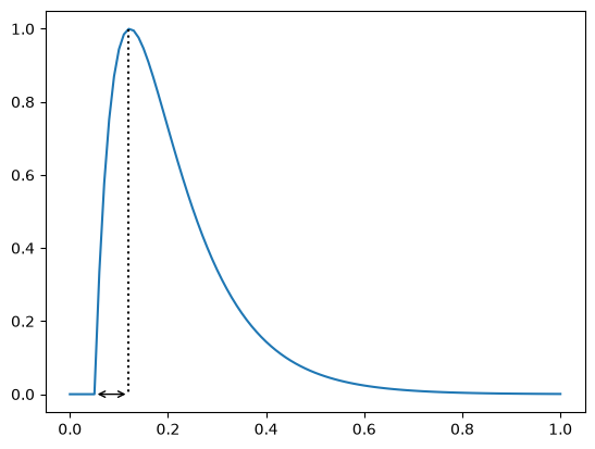
Time to peak#
Time to peak is the time to the maximum attained value of the trace
If no more information than the time stamps and the trace is available, the algorithm will compute the time from the first time stamp (here 0.0) to the time of the maximum attained value
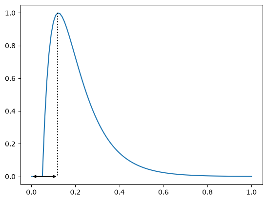
In this case we have
print(apf.features.time_to_peak(y=y, x=time))
0.12
However, if we have pacing information available we can extract information about when the upstroke starts
In which case we have for this trace
print(apf.features.time_to_peak(y=y, x=time, pacing=pacing))
0.06999999999999999
or using the beat object
beat.ttp(use_pacing=True)
np.float64(0.06999999999999999)
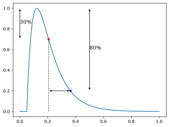
Action potential duration (APD)#
To compute the action potential duration, commonly abbreviated as APD, you first need to find the points when your trace intersects with the APD\(p\) - line and then compute the time difference between those two intersections. For example, say if you want to compute APD30, then you need to find the two intersecting points of the APD30-line which is where you are 30% from the peak of the trace. Once you have found those two intersections you can compute the time difference between those two points.
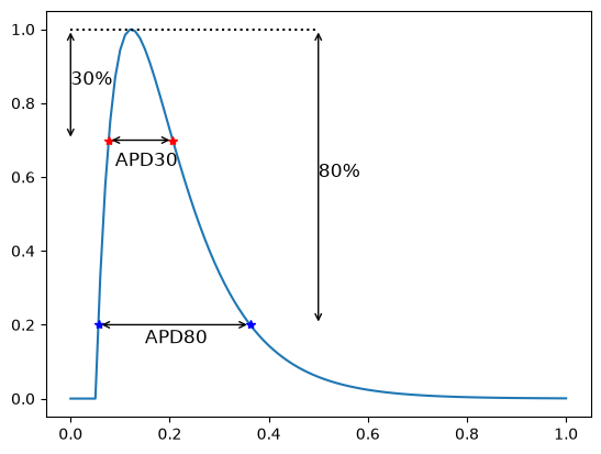
Here we show the APD30 and APD80 which in this case is
print(f"ADP30 = {apf.features.apd(30, y, time)}")
print(f"ADP80 = {apf.features.apd(80, y, time)}")
ADP30 = 0.12940912122129322
ADP80 = 0.3059229823735669
or using the beat object
print(f"ADP30 = {beat.apd(30)}")
print(f"ADP80 = {beat.apd(80)}")
ADP30 = 0.12940912122129322
ADP80 = 0.3059229823735669
Decay time (\(\tau\))#
The decay time, also referred to as \(\tau_p\) (for some \(p\)) is the time from the attained peak value to the intersection of the APD \(p\)-line occurring after the peak value (i.e during the repolarization)
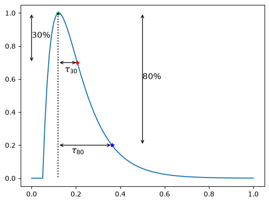
Here you see the \(\tau_{30}\) and \(\tau_{80}\) which in this case is
print(f"\u03c4_30 = {apf.features.tau(a=30, y=y, x=time)}")
print(f"\u03c4_80 = {apf.features.tau(a=80, y=y, x=time)}")
τ_30 = 0.1951680427731784
τ_80 = 0.06484277207692196
or using the beat object
print(f"\u03c4_30 = {beat.tau(30)}")
print(f"\u03c4_80 = {beat.tau(80)}")
τ_30 = 0.1951680427731784
τ_80 = 0.06484277207692196
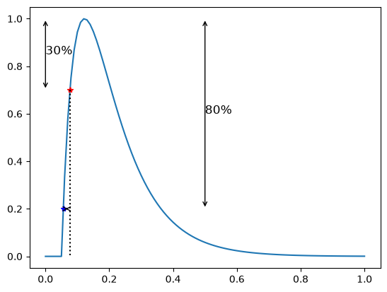
Upstroke time#
The upstroke time is the time from the first intersection of the APD \(p\)-line occurring before the peak value (i.e during the depolarization) to the attained peak value
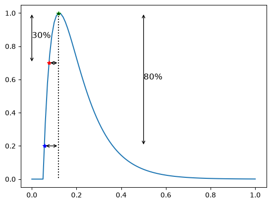
The upstroke time in this case is
print(f"Upstroke 30 = {apf.features.upstroke(a=30, y=y, x=time)}")
print(f"Upstroke 80 = {apf.features.upstroke(a=80, y=y, x=time)}")
Upstroke 30 = 0.04328364176313941
Upstroke 80 = 0.06358780310936087
or equivalently
print(f"Upstroke 30 = {beat.upstroke(a=30)}")
print(f"Upstroke 80 = {beat.upstroke(a=80)}")
Upstroke 30 = 0.04328364176313941
Upstroke 80 = 0.06358780310936087
Triangulation#
For \(\tau_p\) we take the time from the peak value to the intersection of the APD \(p\) line during the repolarization. Instead of starting from the \(p\) value we can start from another APD \(q\)-line, e.g we can compute the time from the APD30 line to the APD 80 line during the repolarization. This is called the triangulation 80-30
print(f"Triangulation 30-80 = {apf.features.triangulation(low=30, high=80, V=y, t=time)}")
Triangulation 30-80 = 0.15620969980605223
or using the beat object
print(f"Triangulation 30-80 = {beat.triangulation(low=30, high=80)}")
Triangulation 30-80 = 0.15620969980605223
APD up xy#
This feature takes two factors \(p_1\) and \(p_2\) and report the time from the first intersection of the \(APD\) \(p_1\) line to the first intersection of the \(p_2\)-line. This is equivalent to the upstroke time when \(p_2 = 0\).
print(f"APD upstroke 30-80 = {apf.features.apd_up_xy(low=30, high=80, y=y, t=time)}")
APD upstroke 30-80 = 0.024500577259997706
or using the beat object
print(f"APD upstroke 30-80 = {beat.apd_up_xy(low=30, high=80)}")
APD upstroke 30-80 = 0.024500577259997706