Copyright (C) 2022 Jørgen Schartum Dokken

This file is part of Oasisx SPDX-License-Identifier: MIT

Efficient assembly

This demo illustrates the performance differences between matrix free and cached assembly for the Crank Nicholson time discretization with the implicit Adams-Bashforth linearization in the tentative velocity step of the Navier-Stokes Equation.

We start by importing the necessary modules

import seaborn
import pandas
import dolfinx
import dolfinx.fem.petsc
from mpi4py import MPI
from petsc4py import PETSc
import ufl
import numpy as np

We define a function, that takes in a mesh, the order P of the Lagrange function space for the scalar component of the velocity field, the number of times we should time the assembly, and jit_options for just in time compilation of the vartiational forms.

For the Matrix-vector strategy, we do only time the time it takes to modify the pre-assembled convection matrix, adding the scaled mass and stiffness matrices and computing the matrix vector product, as the matrix A is needed for the LHS assembly in the fractional step method.

For the Action strategy we use ufl.action to create the variational form for the RHS vector, and use generated code for the assembly.

This demo does not consider any Dirichet boundary conditions.

We add some arbitrary data to the variables dt, nu, u_1 and u_ab, as we are not solving a full problem here.

def assembly(mesh, P: int, repeats: int, jit_options: dict = None):
    V = dolfinx.fem.functionspace(mesh, ("Lagrange", int(P)))
    dt = 0.5
    nu = 0.3
    u = ufl.TrialFunction(V)
    v = ufl.TestFunction(V)

    # Solution from previous time step
    u_1 = dolfinx.fem.Function(V)
    u_1.interpolate(lambda x: np.sin(x[0])*np.cos(x[1]))

    # Define variational forms
    mass = ufl.inner(u, v) * ufl.dx
    stiffness = ufl.inner(ufl.grad(u), ufl.grad(v)) * ufl.dx

    u_ab = [dolfinx.fem.Function(V, name=f"u_ab{i}") for i in range(mesh.geometry.dim)]
    convection = ufl.inner(ufl.dot(ufl.as_vector(u_ab), ufl.nabla_grad(u)), v) * ufl.dx
    for u_abi in u_ab:
        u_abi.interpolate(lambda x: x[0])

    # Compile forms for matrix vector products
    jit_options = {} if jit_options is None else jit_options
    mass_form = dolfinx.fem.form(mass, jit_options=jit_options)
    stiffness_form = dolfinx.fem.form(stiffness, jit_options=jit_options)
    convection_form = dolfinx.fem.form(convection, jit_options=jit_options)

    # Compile form for vector assembly (action)
    dt_inv = dolfinx.fem.Constant(mesh, 1./dt)
    dt_inv.name = "dt_inv"
    nu_c = dolfinx.fem.Constant(mesh, nu)
    nu_c.name = "nu"
    lhs = dt_inv * mass - 0.5 * nu_c * stiffness - 0.5*convection
    lhs = dolfinx.fem.form(ufl.action(lhs, u_1), jit_options=jit_options)

    # Assemble time independent matrices
    # Mass matrix
    M = dolfinx.fem.petsc.create_matrix(mass_form)
    M.setOption(PETSc.Mat.Option.SYMMETRIC, True)
    M.setOption(PETSc.Mat.Option.SYMMETRY_ETERNAL, True)
    M.setOption(PETSc.Mat.Option.IGNORE_ZERO_ENTRIES, True)
    dolfinx.fem.petsc.assemble_matrix(M, mass_form)
    M.assemble()
    M.setOption(PETSc.Mat.Option.NEW_NONZERO_LOCATIONS, False)

    # Stiffness matrix
    K = dolfinx.fem.petsc.create_matrix(stiffness_form)
    K.setOption(PETSc.Mat.Option.SYMMETRIC, True)
    K.setOption(PETSc.Mat.Option.SYMMETRY_ETERNAL, True)
    K.setOption(PETSc.Mat.Option.IGNORE_ZERO_ENTRIES, True)
    dolfinx.fem.petsc.assemble_matrix(K, stiffness_form)
    K.assemble()
    K.setOption(PETSc.Mat.Option.NEW_NONZERO_LOCATIONS, False)

    # Create time dependent matrix (convection matrix)
    A = dolfinx.fem.petsc.create_matrix(mass_form)
    A.setOption(PETSc.Mat.Option.IGNORE_ZERO_ENTRIES, True)

    # Vector for matrix vector product
    b = dolfinx.fem.Function(V)

    t_matvec = np.zeros((repeats, mesh.comm.size), dtype=np.float64)
    t_action = np.zeros((repeats, mesh.comm.size), dtype=np.float64)
    for i in range(repeats):
        # Zero out time-dependent matrix
        A.zeroEntries()

        # Add convection term
        dolfinx.fem.petsc.assemble_matrix(A, convection_form)
        A.assemble()

        # Do mat-vec operations
        with dolfinx.common.Timer(f"~{P} {i} Matvec strategy") as _:
            A.scale(-0.5)
            A.axpy(1./dt, M)
            A.axpy(-0.5*nu, K)
            A.mult(u_1.vector, b.vector)
            b.x.scatter_forward()

        # Compute the vector without using pre-generated matrices
        b_d = dolfinx.fem.Function(V)
        with dolfinx.common.Timer(f"~{P} {i} Action strategy") as _:
            dolfinx.fem.petsc.assemble_vector(b_d.vector, lhs)
            b_d.x.scatter_reverse(dolfinx.la.InsertMode.add)
            b_d.x.scatter_forward()
        # Compare results
        assert np.allclose(b.x.array, b_d.x.array)

        # Get timings
        matvec = dolfinx.common.timing(f"~{P} {i} Matvec strategy")
        action = dolfinx.common.timing(f"~{P} {i} Action strategy")
        t_matvec[i, :] = mesh.comm.allgather(matvec[1])
        t_action[i, :] = mesh.comm.allgather(action[1])

    return V.dofmap.index_map_bs * V.dofmap.index_map.size_global, t_matvec, t_action

We solve the problem on a unit cube that is split into tetrahedras with Nx,Ny and Nx tetrahera in the x, y and z-direction respectively.

def run_parameter_sweep(Nx: int, Ny: int, Nz: int, repeats: int, min_degree: int,
                        max_degree: int) -> dict:
    # Information regarding optimization flags can be found at:
    # https://gcc.gnu.org/onlinedocs/gcc/Optimize-Options.html
    jit_options = {"cffi_extra_compile_args": ["-march=native", "-O3"]}

    mesh = dolfinx.mesh.create_unit_cube(MPI.COMM_WORLD, Nx, Ny, Nz)
    Ps = np.arange(min_degree, max_degree+1, dtype=np.int32)
    j = 0
    results = {}
    for i, P in enumerate(Ps):
        dof, matvec, action = assembly(mesh, P, repeats=repeats, jit_options=jit_options)
        for row in matvec:
            for process in row:
                results[j] = {"P": P, "num_dofs": dof, "method":
                              "matvec", "time (s)": process, "procs": MPI.COMM_WORLD.size}
                j += 1
        for row in action:
            for process in row:
                results[j] = {"P": P, "num_dofs": dof, "method":
                              "action", "time (s)": process, "procs": MPI.COMM_WORLD.size}
                j += 1
    return results

We use pandas and seaborn to visualize the results

def create_plot(results: dict, outfile: str):
    if MPI.COMM_WORLD.rank == 0:
        df = pandas.DataFrame.from_dict(results, orient="index")
        df["label"] = "P" + df["P"].astype(str) + " " + \
            df["num_dofs"].astype(str) + " \n Comms: " + df["procs"].astype(str)
        plot = seaborn.catplot(data=df, kind="swarm",  x="label", y="time (s)", hue="method")
        plot.set(yscale="log")
        import matplotlib.pyplot as plt
        plt.grid()
        plt.savefig(outfile)

We start by running the comparison for an increasing number of degrees of freedom on a fixed grid.

if __name__ == "__main__":
    results_p = run_parameter_sweep(30, 25, 23, repeats=3, min_degree=1, max_degree=4)
    create_plot(results_p, "P_sweep.png")

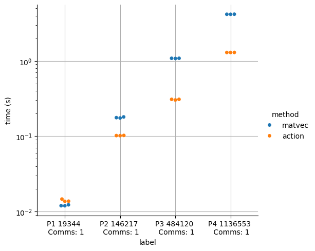
We observe that for all the runs, independent of the degree \(P\), the Action Strategy is significantly faster than the

We note that the run for \(P=1\) is relatively small, and therefore run \(P=1\) on a larger mesh

if __name__ == "__main__":
    results_p1 = run_parameter_sweep(50, 40, 45, 3, 1, 1)
    create_plot(results_p1, "P1.png")

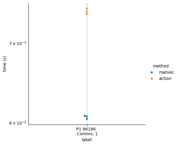
We observe that the run-time of both strategies for \(P = 1\) are more or less the same for larger matrices.