Filtering#
In this notebooks we will explore the effect of filtering resulting motion vectors.
When running the optical flow algorithm to estimate displacement, we find the displacement at each pixel in the image. Some pixels are located in regions without cells we will therefore have very low displacements. However, noise and drift in the images can still give artificial velocity vectors in these pixels.
Displacement vectors that does not contains cells should therefore be filtered out, and we can do so by creating a mask that contains pixels with a significant high displacement.
Let us load the sample dataset and show what we mean
import dataset
import mps_motion
import matplotlib.pyplot as plt

full_resolution = False
data = dataset.load_sample_data(full_resolution=full_resolution)
Download data to /home/runner/work/automatic-motion-estimation/automatic-motion-estimation/notebooks/data/Count00000_Point2C_ChannelBF_Seq0015.npy: 0%| | 0.00/42.0M [00:00<?, ?iB/s]
Download data to /home/runner/work/automatic-motion-estimation/automatic-motion-estimation/notebooks/data/Count00000_Point2C_ChannelBF_Seq0015.npy: 2%|▏ | 1.02M/42.0M [00:00<00:36, 1.11MiB/s]
Download data to /home/runner/work/automatic-motion-estimation/automatic-motion-estimation/notebooks/data/Count00000_Point2C_ChannelBF_Seq0015.npy: 7%|▋ | 3.07M/42.0M [00:01<00:11, 3.47MiB/s]
Download data to /home/runner/work/automatic-motion-estimation/automatic-motion-estimation/notebooks/data/Count00000_Point2C_ChannelBF_Seq0015.npy: 10%|▉ | 4.10M/42.0M [00:01<00:08, 4.21MiB/s]
Download data to /home/runner/work/automatic-motion-estimation/automatic-motion-estimation/notebooks/data/Count00000_Point2C_ChannelBF_Seq0015.npy: 17%|█▋ | 7.17M/42.0M [00:01<00:04, 8.04MiB/s]
Download data to /home/runner/work/automatic-motion-estimation/automatic-motion-estimation/notebooks/data/Count00000_Point2C_ChannelBF_Seq0015.npy: 24%|██▍ | 10.2M/42.0M [00:01<00:02, 11.2MiB/s]
Download data to /home/runner/work/automatic-motion-estimation/automatic-motion-estimation/notebooks/data/Count00000_Point2C_ChannelBF_Seq0015.npy: 32%|███▏ | 13.3M/42.0M [00:01<00:02, 13.8MiB/s]
Download data to /home/runner/work/automatic-motion-estimation/automatic-motion-estimation/notebooks/data/Count00000_Point2C_ChannelBF_Seq0015.npy: 39%|███▉ | 16.4M/42.0M [00:01<00:01, 15.7MiB/s]
Download data to /home/runner/work/automatic-motion-estimation/automatic-motion-estimation/notebooks/data/Count00000_Point2C_ChannelBF_Seq0015.npy: 46%|████▋ | 19.5M/42.0M [00:01<00:01, 17.1MiB/s]
Download data to /home/runner/work/automatic-motion-estimation/automatic-motion-estimation/notebooks/data/Count00000_Point2C_ChannelBF_Seq0015.npy: 54%|█████▎ | 22.5M/42.0M [00:02<00:01, 18.2MiB/s]
Download data to /home/runner/work/automatic-motion-estimation/automatic-motion-estimation/notebooks/data/Count00000_Point2C_ChannelBF_Seq0015.npy: 61%|██████ | 25.6M/42.0M [00:02<00:00, 18.9MiB/s]
Download data to /home/runner/work/automatic-motion-estimation/automatic-motion-estimation/notebooks/data/Count00000_Point2C_ChannelBF_Seq0015.npy: 68%|██████▊ | 28.7M/42.0M [00:02<00:00, 19.6MiB/s]
Download data to /home/runner/work/automatic-motion-estimation/automatic-motion-estimation/notebooks/data/Count00000_Point2C_ChannelBF_Seq0015.npy: 76%|███████▌ | 31.7M/42.0M [00:02<00:00, 20.0MiB/s]
Download data to /home/runner/work/automatic-motion-estimation/automatic-motion-estimation/notebooks/data/Count00000_Point2C_ChannelBF_Seq0015.npy: 83%|████████▎ | 34.8M/42.0M [00:02<00:00, 20.2MiB/s]
Download data to /home/runner/work/automatic-motion-estimation/automatic-motion-estimation/notebooks/data/Count00000_Point2C_ChannelBF_Seq0015.npy: 90%|█████████ | 37.9M/42.0M [00:02<00:00, 20.3MiB/s]
Download data to /home/runner/work/automatic-motion-estimation/automatic-motion-estimation/notebooks/data/Count00000_Point2C_ChannelBF_Seq0015.npy: 98%|█████████▊| 41.0M/42.0M [00:02<00:00, 20.2MiB/s]
Download data to /home/runner/work/automatic-motion-estimation/automatic-motion-estimation/notebooks/data/Count00000_Point2C_ChannelBF_Seq0015.npy: 100%|██████████| 42.0M/42.0M [00:02<00:00, 14.0MiB/s]
Now, let us rus the optical flow algorithm to find the displacements
opt_flow = mps_motion.OpticalFlow(data, flow_algorithm="farneback")
u = opt_flow.get_displacements()
2024-10-14 14:29:18,252 [1887] INFO mps_motion.farneback: Get displacements using Farneback's algorithm
[ ] | 0% Completed | 201.02 us
[# ] | 3% Completed | 103.59 ms
[#### ] | 10% Completed | 204.37 ms
[###### ] | 15% Completed | 305.08 ms
[######## ] | 20% Completed | 405.76 ms
[########## ] | 25% Completed | 506.47 ms
[############ ] | 30% Completed | 607.23 ms
[############## ] | 36% Completed | 708.78 ms
[################ ] | 41% Completed | 809.72 ms
[################## ] | 47% Completed | 910.45 ms
[##################### ] | 52% Completed | 1.01 s
[####################### ] | 57% Completed | 1.11 s
[######################### ] | 62% Completed | 1.21 s
[########################### ] | 67% Completed | 1.31 s
[############################# ] | 73% Completed | 1.41 s
[############################### ] | 78% Completed | 1.51 s
[################################# ] | 84% Completed | 1.62 s
[################################### ] | 89% Completed | 1.72 s
[##################################### ] | 94% Completed | 1.82 s
[########################################] | 100% Completed | 1.92 s
2024-10-14 14:29:20,366 [1887] INFO mps_motion.farneback: Done running Farneback's algorithm
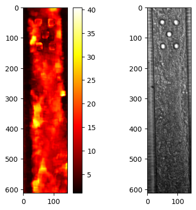
Now let ut compute the maximum displacement norm for each pixel
u_norm_max = u.norm().max().compute()
fig, ax = plt.subplots(1, 2)
im = ax[0].imshow(u_norm_max, cmap="hot")
fig.colorbar(im, ax=ax[0])
ax[1].imshow(data.frames[:, :, 0], cmap="gray")
plt.show()
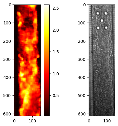
As we can see, some regions without cells have very low displacements. This also includes that pilars.
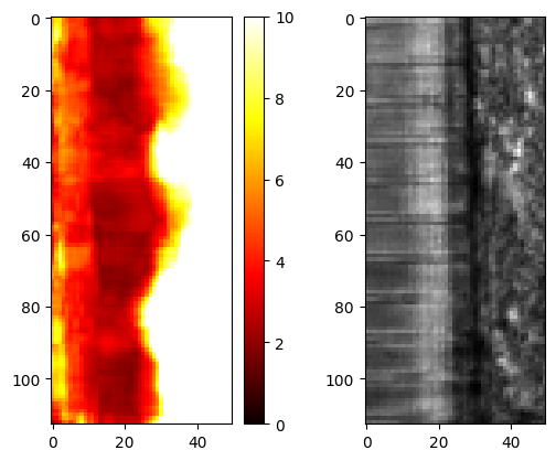
Now let us zoom in at the lower left corner of the image, where we have the fenestrations. These pixels does not contain any cells so these pixels should have zero displacement
fig, ax = plt.subplots(1, 2)
im = ax[0].imshow(u_norm_max[500:, :50], cmap="hot", vmin=0, vmax=0.25)
fig.colorbar(im, ax=ax[0])
ax[1].imshow(data.frames[500:, :50, 0], cmap="gray")
plt.show()
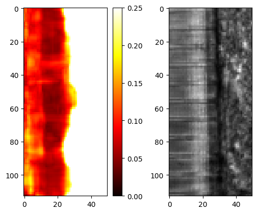
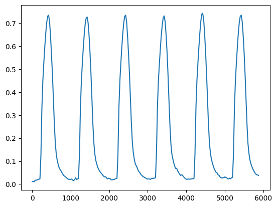
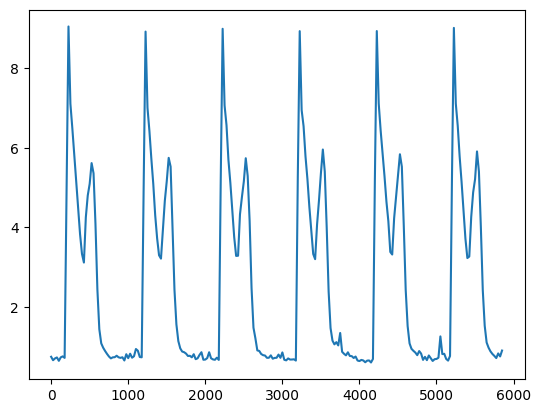
However, we see that displacement are not zero, but slightly positive. For reference let us also compute the average trace over time
u_norm_mean = u.norm().mean().compute()
fig, ax = plt.subplots()
ax.plot(data.time_stamps, u_norm_mean)
plt.show()
Now let ut do the same with the velocity
# We multiply be 1000 to convert from um/ms to um/s
v = opt_flow.get_velocities() * 1000
v_norm_max = v.norm().max().compute()
2024-10-14 14:29:21,821 [1887] INFO mps_motion.farneback: Get velocities using Farneback's algorithm
[ ] | 0% Completed | 169.58 us
[# ] | 4% Completed | 103.14 ms
[#### ] | 10% Completed | 203.84 ms
[###### ] | 16% Completed | 304.65 ms
[######## ] | 22% Completed | 405.51 ms
[########### ] | 27% Completed | 506.30 ms
[############# ] | 33% Completed | 606.96 ms
[############### ] | 39% Completed | 707.76 ms
[################## ] | 45% Completed | 808.65 ms
[#################### ] | 51% Completed | 909.68 ms
[###################### ] | 57% Completed | 1.01 s
[######################## ] | 62% Completed | 1.11 s
[########################### ] | 68% Completed | 1.21 s
[############################# ] | 74% Completed | 1.31 s
[################################ ] | 80% Completed | 1.42 s
[################################## ] | 85% Completed | 1.52 s
[#################################### ] | 91% Completed | 1.62 s
[###################################### ] | 97% Completed | 1.72 s
[########################################] | 100% Completed | 1.82 s
2024-10-14 14:29:23,842 [1887] INFO mps_motion.farneback: Done running Farneback's algorithm
fig, ax = plt.subplots(1, 2)
im = ax[0].imshow(v_norm_max, cmap="hot")
fig.colorbar(im, ax=ax[0])
ax[1].imshow(data.frames[:, :, 0], cmap="gray")
plt.show()
fig, ax = plt.subplots(1, 2)
im = ax[0].imshow(v_norm_max[500:, :50], cmap="hot", vmin=0, vmax=10)
fig.colorbar(im, ax=ax[0])
ax[1].imshow(data.frames[500:, :50, 0], cmap="gray")
plt.show()
And we can see that this effect is amplified in the velocities. Let us compute the average trace over time
v_norm_mean = v.norm().mean().compute()
fig, ax = plt.subplots()
ax.plot(data.time_stamps[:-1], v_norm_mean)
plt.show()
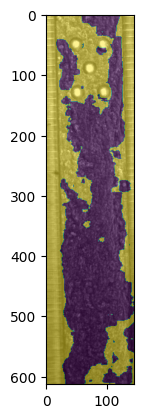
What we can do, is to create a mask where pixels with low displacements are excluded. For simplicity let us exclude all pixels that have a lower value than the mean displacements
mask = u_norm_max < u_norm_max.mean()

fig, ax = plt.subplots()
ax.imshow(data.frames[:, :, 0], cmap="gray")
ax.imshow(mask, alpha=0.5)
plt.show()
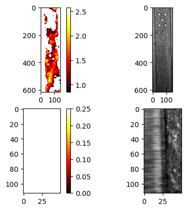
Now let us apply this mask to u and v and repeat the process
u.apply_mask(mask)
v.apply_mask(mask)
u_filtered_norm_max = u.norm().max().compute()

fig, ax = plt.subplots(2, 2)
im = ax[0, 0].imshow(u_filtered_norm_max, cmap="hot")
fig.colorbar(im, ax=ax[0, 0])
ax[0, 1].imshow(data.frames[:, :, 0], cmap="gray")
im = ax[1, 0].imshow(u_filtered_norm_max[500:, :50], cmap="hot", vmin=0, vmax=0.25)
fig.colorbar(im, ax=ax[1, 0])
ax[1, 1].imshow(data.frames[500:, :50, 0], cmap="gray")
plt.show()
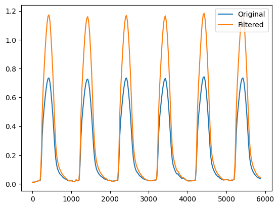
u_filtered_norm_mean = u.norm().mean().compute()
fig, ax = plt.subplots()
ax.plot(data.time_stamps, u_norm_mean, label="Original")
ax.plot(data.time_stamps, u_filtered_norm_mean, label="Filtered")
ax.legend()
plt.show()
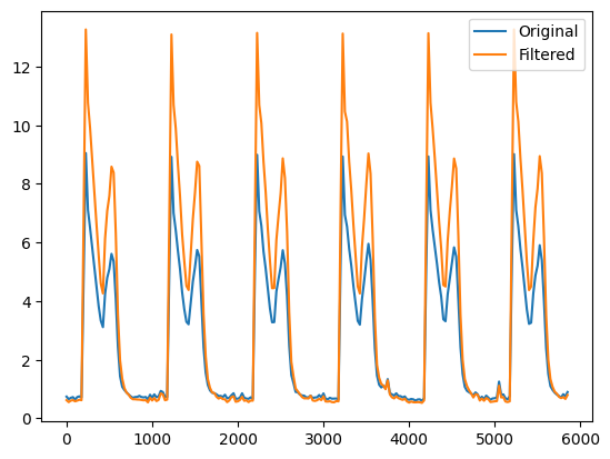
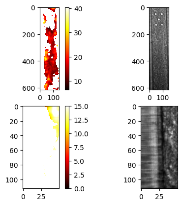
And for the velocity
v_filtered_norm_max = v.norm().max().compute()

fig, ax = plt.subplots(2, 2)
im = ax[0, 0].imshow(v_filtered_norm_max, cmap="hot")
fig.colorbar(im, ax=ax[0, 0])
ax[0, 1].imshow(data.frames[:, :, 0], cmap="gray")
im = ax[1, 0].imshow(v_filtered_norm_max[500:, :50], cmap="hot", vmin=0, vmax=15)
fig.colorbar(im, ax=ax[1, 0])
ax[1, 1].imshow(data.frames[500:, :50, 0], cmap="gray")
plt.show()
v_filtered_norm_mean = v.norm().mean().compute()
fig, ax = plt.subplots()
ax.plot(data.time_stamps[:-1], v_norm_mean, label="Original")
ax.plot(data.time_stamps[:-1], v_filtered_norm_mean, label="Filtered")
ax.legend()
plt.show()