Mean traces#
In this notebook we will reproduce part of Figure 2 in the paper which compted the average displacement and velocity and performs a background correction of the traces. First we import the necessary packages
import matplotlib.pyplot as plt
from pathlib import Path
import ap_features as apf
import numpy as np
import mps
import mps_motion
from mps_motion import (
    Mechanics,
    OpticalFlow,
)


import dataset
And load the sample dataset
full_resolution = False
data = dataset.load_sample_data(full_resolution=full_resolution)
Next we will create an optical flow object and specify that we want to use the Farnebäck method
opt_flow = mps_motion.OpticalFlow(data, flow_algorithm="farneback")
Now we will compute the displacements
u = opt_flow.get_displacements()
2024-10-14 14:29:35,075 [1928] INFO mps_motion.farneback: Get displacements using Farneback's algorithm
[ ] | 0% Completed | 463.81 us
[# ] | 3% Completed | 103.69 ms
[### ] | 9% Completed | 205.46 ms
[##### ] | 14% Completed | 306.21 ms
[####### ] | 19% Completed | 406.95 ms
[########## ] | 25% Completed | 507.68 ms
[############ ] | 30% Completed | 608.35 ms
[############## ] | 35% Completed | 709.03 ms
[################ ] | 41% Completed | 809.81 ms
[################## ] | 46% Completed | 910.58 ms
[#################### ] | 51% Completed | 1.01 s
[###################### ] | 57% Completed | 1.11 s
[######################### ] | 62% Completed | 1.21 s
[########################### ] | 67% Completed | 1.31 s
[############################# ] | 72% Completed | 1.41 s
[############################### ] | 78% Completed | 1.52 s
[################################# ] | 83% Completed | 1.62 s
[################################### ] | 88% Completed | 1.72 s
[##################################### ] | 94% Completed | 1.82 s
[########################################] | 100% Completed | 1.92 s
2024-10-14 14:29:37,198 [1928] INFO mps_motion.farneback: Done running Farneback's algorithm
Lets us inspect the object we got back first
u
VectorFrameSequence((613, 145, 236, 2), dx=1.08615103979884, scale=1.0)
We see that we got a VectorFrameSequence, which is essentially a sequence of frames with a vector, representing the x and y component of the displacement at each point. To convert this into a trace we need to reduce it along some dimension. For example, we could take the norm at each pixel
u_norm = u.norm()
u_norm
FrameSequence((613, 145, 236), dx=1.08615103979884, scale=1.0)
Which gives us a FrameSequence, i.e a sequence of frames with a scalar value at each pixel. Next thing we will do is to reduce each frame to a number, and we can do this by takeing the average value
u_norm_mean = u_norm.mean()
u_norm_mean
|
||||||||||||||||
As we can see we get a dask array back. These are similar to numpy array, but much more memory efficient and we can also perform operations on them in parallel. To get the actual value, we need to call compute.
u_norm_mean_array = u_norm_mean.compute()
u_norm_mean_array
array([0.01133613, 0.01181203, 0.01092554, 0.01695736, 0.01735373,
       0.01825244, 0.02097465, 0.0216327 , 0.02340233, 0.12392896,
       0.32805845, 0.44829714, 0.5263814 , 0.59549445, 0.6549505 ,
       0.70148593, 0.72976124, 0.73448515, 0.7058238 , 0.6423673 ,
       0.5625425 , 0.47395515, 0.36719313, 0.25677645, 0.1742699 ,
       0.12830646, 0.10206641, 0.08470403, 0.07076644, 0.06325455,
       0.05731892, 0.04886169, 0.04202039, 0.03634347, 0.03397745,
       0.02992143, 0.02598923, 0.02285744, 0.02103288, 0.02097288,
       0.02124553, 0.02225307, 0.01722706, 0.01630166, 0.01912291,
       0.02762973, 0.02030424, 0.02246259, 0.02452746, 0.12531026,
       0.32627264, 0.44562453, 0.52298474, 0.59150773, 0.65124226,
       0.6958776 , 0.7221573 , 0.7264151 , 0.7017745 , 0.646587  ,
       0.5708046 , 0.478316  , 0.3691665 , 0.25808898, 0.17845234,
       0.13145462, 0.10322256, 0.08743887, 0.07374295, 0.06430505,
       0.05680412, 0.0505007 , 0.04600941, 0.04094174, 0.03515033,
       0.03194215, 0.03266467, 0.02860973, 0.0231214 , 0.02610733,
       0.02411683, 0.0235027 , 0.01875073, 0.01895361, 0.02057876,
       0.01995521, 0.02259676, 0.02414181, 0.02582131, 0.12969515,
       0.33215576, 0.44823006, 0.524528  , 0.5938487 , 0.65422577,
       0.6999275 , 0.72958064, 0.7343337 , 0.7049523 , 0.642895  ,
       0.5662173 , 0.4763548 , 0.36693588, 0.25972313, 0.17878495,
       0.135004  , 0.10763776, 0.08928484, 0.07994022, 0.07133472,
       0.06045376, 0.05325934, 0.04859821, 0.04124243, 0.03775689,
       0.03278338, 0.03127093, 0.02776042, 0.02688984, 0.02267595,
       0.02257306, 0.02324977, 0.02191778, 0.02136647, 0.0256929 ,
       0.02470831, 0.02583716, 0.02617044, 0.02866017, 0.13333264,
       0.3339685 , 0.44831318, 0.52189225, 0.5866564 , 0.64603573,
       0.6909387 , 0.7229275 , 0.7311511 , 0.70691377, 0.6495675 ,
       0.5737323 , 0.47674313, 0.36259422, 0.25708747, 0.17533831,
       0.13156988, 0.10992262, 0.09212036, 0.07721698, 0.0684281 ,
       0.06923591, 0.05806442, 0.0507962 , 0.04390529, 0.03811287,
       0.04035631, 0.03921758, 0.03284859, 0.02865543, 0.02354487,
       0.02168579, 0.02109195, 0.02253222, 0.02181454, 0.02182607,
       0.02282436, 0.02283431, 0.02421736, 0.025817  , 0.13038199,
       0.3307728 , 0.44728976, 0.52256167, 0.59047   , 0.65390825,
       0.70496964, 0.7385412 , 0.7425983 , 0.7163383 , 0.6552204 ,
       0.57714427, 0.48170748, 0.37154582, 0.26183566, 0.18134323,
       0.13597763, 0.1104297 , 0.09255202, 0.07929214, 0.06698784,
       0.05870654, 0.05089182, 0.04898664, 0.04040511, 0.03833683,
       0.03147116, 0.02907328, 0.0264352 , 0.02823776, 0.02835899,
       0.03140689, 0.02941639, 0.02757149, 0.02400329, 0.02270887,
       0.02598018, 0.02401981, 0.02807213, 0.03012623, 0.1310668 ,
       0.3324555 , 0.44940254, 0.52596027, 0.5941578 , 0.6550852 ,
       0.70200115, 0.7290153 , 0.7345981 , 0.7083933 , 0.65105   ,
       0.57434195, 0.48171267, 0.37095428, 0.26168576, 0.17943421,
       0.13483599, 0.10714342, 0.09017489, 0.07779691, 0.06698018,
       0.05886999, 0.05121228, 0.04477327, 0.04149215, 0.04008143,
       0.03767776], dtype=float32)
We can now plot the array
fig, ax = plt.subplots()
ax.plot(data.time_stamps, u_norm_mean_array)
ax.set_xlabel("Time (s)")
ax.set_ylabel("Displacement (\u00B5m)")
plt.show()
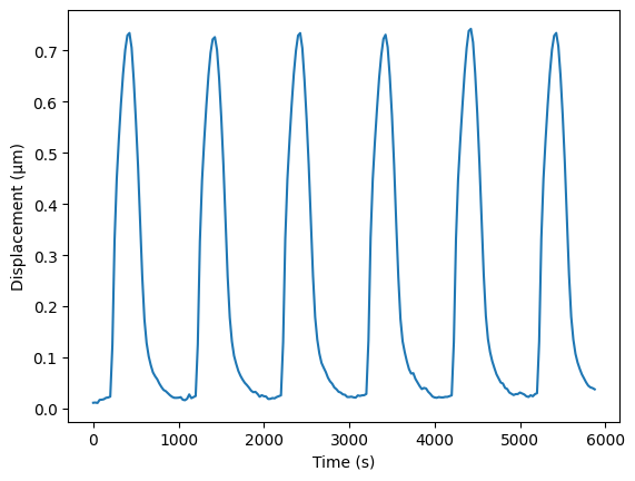
Note that in this case we didn’t specify which frame to use as the reference frame, which means that it will use the first frame. This turns out to work well in this case, but image we for example had chosen frame at time 500 ms (which is approximately at the peak contraction), then we would get
u_20 = opt_flow.get_displacements(reference_frame=500, recompute=True)
u_20_array = u_20.norm().mean().compute()
fig, ax = plt.subplots()
ax.plot(data.time_stamps, u_20_array)
ax.set_ylabel("Displacement (\u00B5m)")
ax.set_xlabel("Time (s)")
plt.show()
2024-10-14 14:29:37,877 [1928] INFO mps_motion.farneback: Get displacements using Farneback's algorithm
[ ] | 0% Completed | 119.51 us
[## ] | 5% Completed | 103.64 ms
[#### ] | 10% Completed | 204.34 ms
[###### ] | 16% Completed | 305.24 ms
[######## ] | 22% Completed | 406.07 ms
[########### ] | 27% Completed | 506.74 ms
[############# ] | 33% Completed | 612.87 ms
[############### ] | 39% Completed | 714.68 ms
[################## ] | 45% Completed | 815.62 ms
[#################### ] | 51% Completed | 916.50 ms
[###################### ] | 56% Completed | 1.02 s
[######################### ] | 63% Completed | 1.12 s
[########################### ] | 67% Completed | 1.22 s
[############################# ] | 72% Completed | 1.32 s
[############################### ] | 79% Completed | 1.42 s
[################################# ] | 84% Completed | 1.52 s
[################################### ] | 89% Completed | 1.62 s
[###################################### ] | 96% Completed | 1.72 s
[########################################] | 100% Completed | 1.82 s
2024-10-14 14:29:39,902 [1928] INFO mps_motion.farneback: Done running Farneback's algorithm
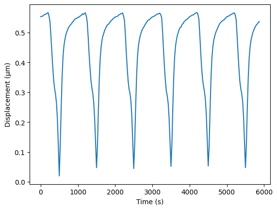
We will see how we can automate the detection of a suitable reference frame later.
First we can also find the velocity trace
v = opt_flow.get_velocities()
v_norm_mean_array = v.norm().mean().compute()

time = data.time_stamps[:-1]

fig, ax = plt.subplots()
ax.plot(time, v_norm_mean_array)
ax.set_xlabel("Time (s)")
ax.set_ylabel("Velocity (\u00B5m/s)")
plt.show()
2024-10-14 14:29:40,528 [1928] INFO mps_motion.farneback: Get velocities using Farneback's algorithm
[ ] | 0% Completed | 378.54 us
[## ] | 5% Completed | 101.11 ms
[#### ] | 10% Completed | 201.81 ms
[###### ] | 15% Completed | 302.77 ms
[######## ] | 22% Completed | 403.69 ms
[########## ] | 27% Completed | 504.38 ms
[############# ] | 33% Completed | 605.33 ms
[############### ] | 39% Completed | 706.17 ms
[################# ] | 44% Completed | 807.03 ms
[#################### ] | 51% Completed | 908.06 ms
[###################### ] | 56% Completed | 1.01 s
[######################### ] | 62% Completed | 1.11 s
[########################### ] | 68% Completed | 1.21 s
[############################# ] | 74% Completed | 1.31 s
[################################ ] | 80% Completed | 1.41 s
[################################## ] | 85% Completed | 1.51 s
[#################################### ] | 91% Completed | 1.61 s
[###################################### ] | 97% Completed | 1.71 s
[########################################] | 100% Completed | 1.82 s
2024-10-14 14:29:42,547 [1928] INFO mps_motion.farneback: Done running Farneback's algorithm
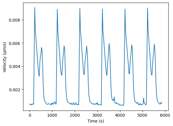
Here it is also worth noting that we have an array that has one less element than the displacement, because the velocity is essentially computing be taking the difference between successive displacements and dividing by the time difference. We could also increase the spacing between the displacement by passing in the spacing argument
v5 = opt_flow.get_velocities(spacing=5)
v5_norm_mean_array = v5.norm().mean().compute()

time = data.time_stamps[:-5]

fig, ax = plt.subplots()
ax.plot(time, v5_norm_mean_array)
ax.set_xlabel("Time (s)")
ax.set_ylabel("Velocity (\u00B5m/s)")
plt.show()
2024-10-14 14:29:43,161 [1928] INFO mps_motion.farneback: Get velocities using Farneback's algorithm
[ ] | 0% Completed | 118.31 us
[## ] | 5% Completed | 101.06 ms
[#### ] | 10% Completed | 201.78 ms
[###### ] | 16% Completed | 302.69 ms
[######### ] | 22% Completed | 403.62 ms
[########### ] | 28% Completed | 504.49 ms
[############# ] | 34% Completed | 605.26 ms
[################ ] | 40% Completed | 706.13 ms
[################## ] | 46% Completed | 806.98 ms
[#################### ] | 52% Completed | 907.83 ms
[####################### ] | 58% Completed | 1.01 s
[######################### ] | 64% Completed | 1.11 s
[############################ ] | 70% Completed | 1.21 s
[############################## ] | 75% Completed | 1.31 s
[################################ ] | 81% Completed | 1.41 s
[################################### ] | 87% Completed | 1.51 s
[##################################### ] | 94% Completed | 1.62 s
[########################################] | 100% Completed | 1.72 s
2024-10-14 14:29:45,074 [1928] INFO mps_motion.farneback: Done running Farneback's algorithm
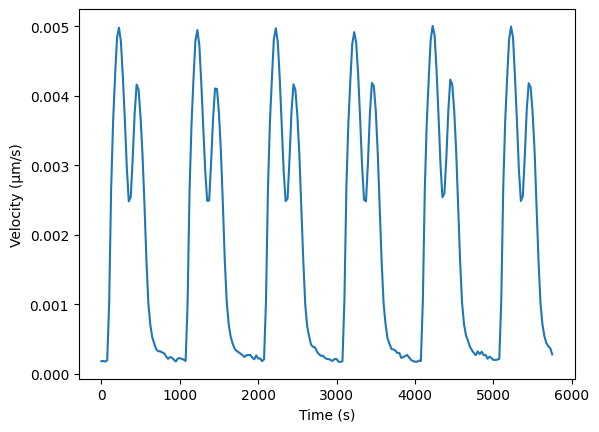
As a consequence we get a more smooth signal. Depending on the framerate of the video you are analyzing you might choose different spacing to avoid too much noise in the velocity traces. For this dataset a spacing of 1.0 seems to be appropriate.
Estimating the reference frame#
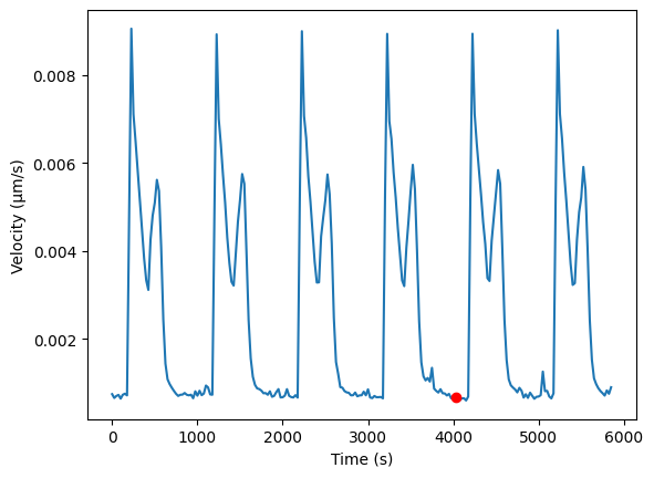
We would like to choose a reference frame where the cells are at rest, which would be equivalent to having (close to) zero velocity. For this we have implemented a helper function to achieve just that.
ref_index = mps_motion.motion_tracking.estimate_referece_image_from_velocity(t=data.time_stamps[:-1], v=v_norm_mean_array)
print(f"Reference index {ref_index} at time {data.time_stamps[ref_index]}")
type(ref_index)
Reference index 161 at time 4025.6679687499854
int
And we see that it found a reference index of 161 and time 4025
fig, ax = plt.subplots()
ax.plot(data.time_stamps[:-1], v_norm_mean_array)
ax.plot([data.time_stamps[ref_index]], [v_norm_mean_array[ref_index]], "ro")
ax.set_xlabel("Time (s)")
ax.set_ylabel("Velocity (\u00B5m/s)")
plt.show()
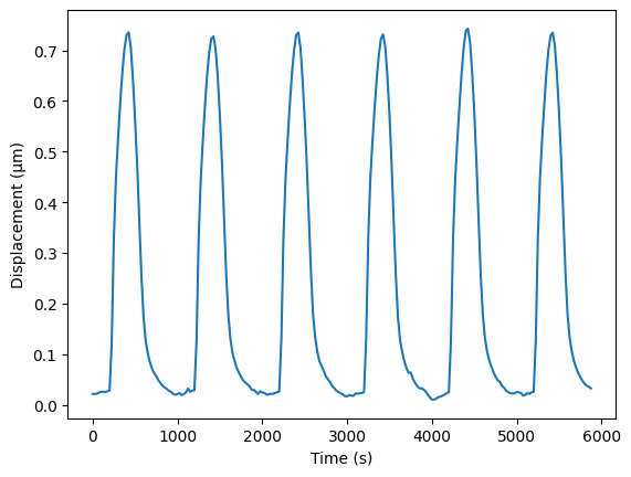
And we can now use this reference index instead for the displacement
u = opt_flow.get_displacements(reference_frame=data.time_stamps[ref_index], recompute=True)
u_array = u.norm().mean().compute()
fig, ax = plt.subplots()
ax.plot(data.time_stamps, u_array)
ax.set_ylabel("Displacement (\u00B5m)")
ax.set_xlabel("Time (s)")
plt.show()
2024-10-14 14:29:45,773 [1928] INFO mps_motion.farneback: Get displacements using Farneback's algorithm
[ ] | 0% Completed | 104.15 us
[## ] | 5% Completed | 101.05 ms
[#### ] | 10% Completed | 201.74 ms
[###### ] | 16% Completed | 302.49 ms
[######## ] | 21% Completed | 403.17 ms
[########### ] | 28% Completed | 503.91 ms
[############# ] | 33% Completed | 604.71 ms
[################ ] | 40% Completed | 705.56 ms
[################## ] | 45% Completed | 806.22 ms
[#################### ] | 52% Completed | 906.97 ms
[###################### ] | 57% Completed | 1.01 s
[######################### ] | 63% Completed | 1.11 s
[########################### ] | 69% Completed | 1.21 s
[############################## ] | 75% Completed | 1.31 s
[################################ ] | 80% Completed | 1.41 s
[################################## ] | 86% Completed | 1.51 s
[##################################### ] | 92% Completed | 1.61 s
[####################################### ] | 98% Completed | 1.71 s
[########################################] | 100% Completed | 1.81 s
2024-10-14 14:29:47,782 [1928] INFO mps_motion.farneback: Done running Farneback's algorithm
Background correction#
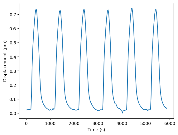
Run running the motion tracking software, some background drift might be cumulated in the resulting displacements. However the displacements at the reference image should be zero. This might lead to a sudden jump in the displacement at the point of reference. To circumvent this, we have an argument called smooth_ref_transition, which by default is set to True. If we set this to false, we see this phenomena more clearly
u_no_smooth = opt_flow.get_displacements(reference_frame=data.time_stamps[ref_index], recompute=True, smooth_ref_transition=False)
u_no_smooth_array = u_no_smooth.norm().mean().compute()
fig, ax = plt.subplots()
ax.plot(data.time_stamps, u_no_smooth_array)
ax.set_ylabel("Displacement (\u00B5m)")
ax.set_xlabel("Time (s)")
plt.show()
2024-10-14 14:29:48,415 [1928] INFO mps_motion.farneback: Get displacements using Farneback's algorithm
[ ] | 0% Completed | 96.54 us
[## ] | 5% Completed | 103.79 ms
[#### ] | 10% Completed | 204.64 ms
[###### ] | 16% Completed | 305.34 ms
[######## ] | 22% Completed | 406.08 ms
[########### ] | 27% Completed | 506.75 ms
[############# ] | 33% Completed | 607.45 ms
[############### ] | 39% Completed | 708.43 ms
[################## ] | 45% Completed | 810.37 ms
[#################### ] | 50% Completed | 911.05 ms
[###################### ] | 57% Completed | 1.01 s
[######################### ] | 62% Completed | 1.11 s
[########################### ] | 68% Completed | 1.21 s
[############################# ] | 74% Completed | 1.31 s
[################################ ] | 80% Completed | 1.42 s
[################################## ] | 86% Completed | 1.52 s
[#################################### ] | 91% Completed | 1.62 s
[####################################### ] | 97% Completed | 1.72 s
[########################################] | 100% Completed | 1.82 s
2024-10-14 14:29:50,429 [1928] INFO mps_motion.farneback: Done running Farneback's algorithm
To remove the background from the trace, we can use a background correction algorithm to first estimate the baseline and then subtract it. This algorithm is implemented in the ap_features library
background = apf.background.correct_background(data.time_stamps, u_array, method="subtract")
fig, ax = plt.subplots(1, 2, figsize=(8, 3))
ax[0].plot(data.time_stamps, u_array)
ax[0].plot(data.time_stamps, background.background)
ax[0].set_ylabel("Displacement (\u00B5m)")
ax[0].set_title("Original with backgorund")
ax[1].plot(data.time_stamps, background.corrected)
ax[1].set_title("Corrected")
Text(0.5, 1.0, 'Corrected')
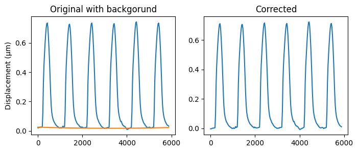
In this base there is not much drift in the signal, but this might occur in other datasets.