Constitutive relations
Contents
Constitutive relations
We have now covered a mechanical framework which holds any for material in general. What differentiate the mechanics of soft living tissue, like the myocardium, from other materials is the constitutive relations which describes the response of a material to applied load. Such constitutive relations often comes from experimental observations, both observations of anatomical structure but also from experiments done on tissue slabs.
We have already covered the theory of hyperelasticity and incompressibility in Section Hyperelasticity and Incompressibility respectively which are types of constitutive relations. In this section we will cover constitutive relations which only apply to soft living tissue such as the myocardium. In particular, we will consider a complete constitutive model of the mechanical behavior of the myocardium that accounts for both the passive and the active response of the myocardium.
Modeling of the passive myocardium
The passive response of the myocardium has been investigated through uni-axial, bi-axial and shear deformation experiments [Dokos et al., 2002].
In 2009 Holzapfel and Ogden proposed an orthotropic constitutive model of the passive myocardium [Holzapfel and Ogden, 2009] which is based on the experiments done in [Dokos et al., 2002], and is the model used in this thesis. Other constitutive models for the passive myocardium exists [Costa et al., 2001, Guccione et al., 1991, Nash and Hunter, 2000] but is not considered here. The model assumes a local orthonormal coordinate system with the fiber axis \(\mathbf{f}_0\), sheet axis \(\mathbf{s}_0\) and sheet-normal axis \(\mathbf{n}_0\).
From this coordinate system we define the invariants
Here \(I_{4\mathbf{f}_0} \) and \(I_{4\mathbf{s}_0}\) are the stretches along the fiber, sheet axis respectively and \(I_{8\mathbf{f}_0\mathbf{s}_0}\) is related to the angle between the fiber and sheets in the current configuration given that they are orthogonal in the reference configuration. Note that since \((\mathbf{f}_0, \mathbf{s}_0, \mathbf{n}_0)\) is an orthonormal system, we have the relation \(I_1 = I_{4\mathbf{f}_0} + I_{4\mathbf{s}_0} +I_{4\mathbf{n}_0}\), and so \(I_{4\mathbf{n}_0}\) is redundant. The orthotropic Holzapfel and Ogden model reads
Here \(( x )_+ = \frac{1}{2} \left( x + |x| \right)\), so that the the terms involving \(I_{4\mathbf{f}_0}\) and \(I_{4\mathbf{s}_0}\) only contribute to the stored energy during elongation. From (20) we see that it is easy to identify the physical meaning of each term. For example the first term represents the isotropic contribution which is the overall stiffness in the extracellular matrix while the second term accounts for the extra stiffness along the fibers when they are elongated. It is also straight forward to prove that the strain-energy function is convex, and that the requirements for existence and uniqueness discussed in General requirements for the strain-energy density function are fulfilled.
In this thesis we have used a transversely isotropic version of (20) which is obtained by setting \(a_{fs} = b_{fs}= a_s = b_s = 0\), i.e
If we further set \(a_f = b_f = b = 0\) so that in \(a\) is the only nonzero parameter, then the Holzapfel-Ogden model reduces (after a series expansion of the exponential and a limiting argument) to
which is the model of a Neo Hookean material. The Cauchy stress can be derived analytically from (20), by using the chain rule and (16),
where \(\mathbf{B} = \mathbf{F} \mathbf{F}^{T}\) is the left Cauchy-Green tensor, \(\mathbf{f} = \mathbf{F} \mathbf{f}_0\) and \(\mathbf{s} = \mathbf{F} \mathbf{s}_0\).
Modeling of the active contraction
One feature that separates the myocardium from other hyperelastic materials such as rubber, is its ability to actively generate force without external loads. This active component of the model can be incorporated using two fundamentally different approaches known as the active stress and active strain formulation.

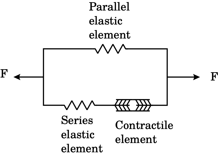
Fig. 2 The classical three-element Hill muscle model with one contractile element and two non-linear springs, one arranged in series and one parallel.
The active stress approach is based on the classical three element Hill model illustrated in Fig. 2, where the active contribution naturally decomposes the total stress into a sum of passive and active stresses [Nash and Panfilov, 2004]. Hence, in the active stress formulation [Hunter et al., 1998] one assumes that the total Cauchy stress \(\sigma\) can be written as an additive sum of one passive contribution \(\sigma_p\) and one active contribution \(\sigma_a\),
The passive contribution is determined by the material model used
while the active contribution is given by
and the different constants \(\sigma_{ff}, \sigma_{ss}\), and \(\sigma_{nn}\), which are the active stress in the fiber, sheet and sheet-normal direction respectively, are typically coupled to the electrophysiology and calcium dynamics. There are experimental evidence that the active stresses in the transverse direction of the fibers (\(\sigma_{ss}\), and \(\sigma_{nn}\)), are non-negligible [Lin and Yin, 1998], and one approach is to assume a uniform transverse activation in which the total active tension can be written as
where \(\eta\) represent the amount of transverse activation and \(T_a \in \mathbb{R}\) is the magnitude of the active tension. In the limiting case (\(\eta = 0.0\)), the active tension acts purely along the fibers and (22) reduces to
Note that, by observing that
and that \(I_1 = I_{4\mathbf{f}_0} + I_{4\mathbf{s}_0} + I_{4\mathbf{n}_0}\), we can instead decompose the strain-energy function into a passive and active parts [Pathmanathan et al., 2010], \(\Psi= \Psi_p + \Psi_a\), with
so that \(J \sigma_a = \frac{\partial \Psi_a}{\partial \mathbf{F}} \mathbf{F}^{T}\).
The active strain formulation is a relatively new way of modeling the active contraction in the heart and was first introduced in [Taber and Perucchio, 2000]. This formulation is based on a multiplicative decomposition of the deformation gradient,
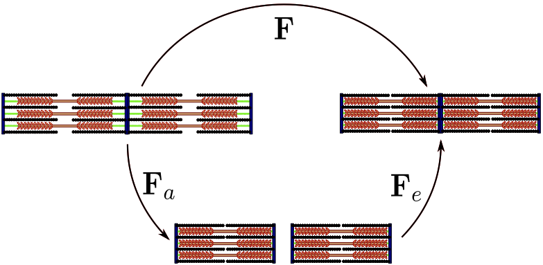
The active part \(\mathbf{F}_a\), is an inelastic process driven by the biochemistry and can be seen as the actual distortion of the microstructure. The elastic part \(\mathbf{F}_e\) is responsible for preserving compatibility of the tissue and stores all the energy in the deformations. As a consequence, the strain energy function is a function of the elastic deformation gradient only. The decoupling can be illustrated by considering two sarcomeres connected in series as shown in Fig. 3.

Fig. 3 Illustration of the active strain formulation. During the active deformation, the sarcomeres shortens as if they were all detached. The elastic deformation ensures compatibility of the tissue.
The general form of the active deformation gradient for a material with an orthotropic active response is given by
We add the constraint \(\mathrm{det} \; (\mathbf{F}_a) = 1\), meaning that the active deformation is volume preserving. Further we assume that the activation is transversely isotropic, so that the sheet and sheet-normal axis is treated in the same way. It is then straight forward to verify that \(\gamma_n = \gamma_s =1- (1-\gamma_f)^{-1/2}\), and we have
where we set \(\gamma = \gamma_f\) for convenience.
While the motivation behind the active stress formulation is purely physiological and based on the classical Hill model shown in Fig. 2, the motivation behind the active strain formulation is more driven by ensuring mathematical robustness. In particular it has been shown [Ambrosi and Pezzuto, 2012] that with the active strain formulation, properties such as frame invariance and rank-one ellipticity is inherited from the strain energy function. In contrast, rank-one ellipticity is not guaranteed for the active stress formulation.
For a more extensive comparison of the active stress and active strain approach we refer to [Ambrosi and Pezzuto, 2012, Giantesio et al., 2017], and for an overview of other methods to model the active contraction we refer to [Goriely, 2017].
References
- AP12(1,2)
D Ambrosi and S Pezzuto. Active stress vs. active strain in mechanobiology: constitutive issues. Journal of Elasticity, 107(2):199–212, 2012.
- CHM01
Kevin D Costa, Jeffrey W Holmes, and Andrew D McCulloch. Modelling cardiac mechanical properties in three dimensions. Philosophical Transactions of the Royal Society of London A: Mathematical, Physical and Engineering Sciences, 359(1783):1233–1250, 2001.
- DSYL02(1,2)
Socrates Dokos, Bruce H Smaill, Alistair A Young, and Ian J LeGrice. Shear properties of passive ventricular myocardium. American Journal of Physiology-Heart and Circulatory Physiology, 283(6):H2650–H2659, 2002.
- GMR17
Giulia Giantesio, Alessandro Musesti, and Davide Riccobelli. A comparison between active strain and active stress in transversely isotropic hyperelastic materials. arXiv preprint arXiv:1709.04977, 2017.
- Gor17
A Goriely. Five ways to model active processes in elastic solids: active forces, active stresses, active strains, active fibers, and active metrics. Mechanics Research Communications, 2017.
- GMW+91
Julius M Guccione, Andrew D McCulloch, LK Waldman, and others. Passive material properties of intact ventricular myocardium determined from a cylindrical model. J Biomech Eng, 113(1):42–55, 1991.
- HO09
Gerhard A Holzapfel and Ray W Ogden. Constitutive modelling of passive myocardium: a structurally based framework for material characterization. Philosophical Transactions of the Royal Society of London A: Mathematical, Physical and Engineering Sciences, 367(1902):3445–3475, 2009.
- HMTK98
PJ Hunter, AD McCulloch, and HEDJ Ter Keurs. Modelling the mechanical properties of cardiac muscle. Progress in biophysics and molecular biology, 69(2):289–331, 1998.
- LY98
DHS Lin and FCP Yin. A multiaxial constitutive law for mammalian left ventricular myocardium in steady-state barium contracture or tetanus. Journal of biomechanical engineering, 120(4):504–517, 1998.
- NH00
Martyn P Nash and Peter J Hunter. Computational mechanics of the heart. Journal of elasticity and the physical science of solids, 61(1-3):113–141, 2000.
- NP04
Martyn P Nash and Alexander V Panfilov. Electromechanical model of excitable tissue to study reentrant cardiac arrhythmias. Progress in biophysics and molecular biology, 85(2):501–522, 2004.
- PCGW10
Pras Pathmanathan, SJ Chapman, DJ Gavaghan, and JP Whiteley. Cardiac electromechanics: the effect of contraction model on the mathematical problem and accuracy of the numerical scheme. Quaterly Journal of Mechanics and Applied Mathematics, 2010.
- TP00
Larry A Taber and Renato Perucchio. Modeling heart development. Journal of elasticity and the physical science of solids, 61(1-3):165–197, 2000.
