Bestel model

In this example we will show the both the pressure and activation model from Bestel et al. [BClementS01].

import logging
import matplotlib.pyplot as plt
import numpy as np
from scipy.integrate import solve_ivp

from circulation import bestel, log

First let us define a time array

log.setup_logging(level=logging.INFO)
t_eval = np.linspace(0, 1, 200)

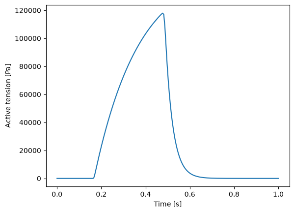
Now we will solve the activation model

activation = bestel.BestelActivation()
result_activation = solve_ivp(
        activation,
        [0, 1],
        [0.0],
        t_eval=t_eval,
        method="Radau",
    )

[11/28/24 20:30:00] INFO     INFO:circulation.bestel:                                                                                                                                       bestel.py:72
                             Bestel activation model                                                                                                                                                    
                                    parameters                                                                                                                                                          
                             ┏━━━━━━━━━━━┳━━━━━━━━━━┓                                                                                                                                                   
                             ┃ Parameter ┃ Value    ┃                                                                                                                                                   
                             ┡━━━━━━━━━━━╇━━━━━━━━━━┩                                                                                                                                                   
                             │ t_sys     │ 0.16     │                                                                                                                                                   
                             │ t_dias    │ 0.484    │                                                                                                                                                   
                             │ gamma     │ 0.005    │                                                                                                                                                   
                             │ a_max     │ 5.0      │                                                                                                                                                   
                             │ a_min     │ -30.0    │                                                                                                                                                   
                             │ sigma_0   │ 150000.0 │                                                                                                                                                   
                             └───────────┴──────────┘                                                                                                                                                   

and plot the results

fig, ax = plt.subplots()
ax.plot(result_activation.t, result_activation.y[0])
ax.set_xlabel("Time [s]")
ax.set_ylabel("Active tension [Pa]")
plt.show()

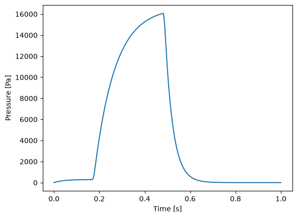
Now we will solve the pressure model

pressure = bestel.BestelPressure()
result_pressure = solve_ivp(
        pressure,
        [0, 1],
        [0.0],
        t_eval=t_eval,
        method="Radau",
    )

                    INFO     INFO:circulation.bestel:                                                                                                                                      bestel.py:177
                              Bestel pressure model                                                                                                                                                     
                                    parameters                                                                                                                                                          
                             ┏━━━━━━━━━━━━┳━━━━━━━━━┓                                                                                                                                                   
                             ┃ Parameter  ┃ Value   ┃                                                                                                                                                   
                             ┡━━━━━━━━━━━━╇━━━━━━━━━┩                                                                                                                                                   
                             │ t_sys_pre  │ 0.17    │                                                                                                                                                   
                             │ t_dias_pre │ 0.484   │                                                                                                                                                   
                             │ gamma      │ 0.005   │                                                                                                                                                   
                             │ a_max      │ 5.0     │                                                                                                                                                   
                             │ a_min      │ -30.0   │                                                                                                                                                   
                             │ alpha_pre  │ 5.0     │                                                                                                                                                   
                             │ alpha_mid  │ 1.0     │                                                                                                                                                   
                             │ sigma_pre  │ 7000.0  │                                                                                                                                                   
                             │ sigma_mid  │ 16000.0 │                                                                                                                                                   
                             └────────────┴─────────┘                                                                                                                                                   

and plot the results

fig, ax = plt.subplots()
ax.plot(result_pressure.t, result_pressure.y[0])
ax.set_xlabel("Time [s]")
ax.set_ylabel("Pressure [Pa]")
plt.show()

References

[BClementS01]

Julie Bestel, Frédérique Clément, and Michel Sorine. A biomechanical model of muscle contraction. In Medical Image Computing and Computer-Assisted Intervention–MICCAI 2001: 4th International Conference Utrecht, The Netherlands, October 14–17, 2001 Proceedings 4, 1159–1161. Springer, 2001.