Zenker#
This example shows how to use the Zenker model [ZRC19]. The Zenker model is a 0D model that simulates the cardiac cycle.
from circulation.log import setup_logging
from circulation.zenker import Zenker
import matplotlib.pyplot as plt
import numpy as np
setup_logging()
circulation = Zenker(
    parameters={
        "start_withdrawal": 100,
        "end_withdrawal": 200,
        "start_infusion": 400,
        "end_infusion": 500,
        "flow_withdrawal": -1,
        "flow_infusion": 1,
        "Vv0_min": 1000,
        "Vv0_max": 2000,
    }
)
history = circulation.solve(T=700.0, dt=1e-3, dt_eval=0.1)
start_plot = 0
time = history["time"][start_plot:]
[06/29/26 20:16:11] INFO     INFO:circulation.base:                                                                                                                                          base.py:134
                                           Circulation model parameters (Zenker)
                             ┏━━━━━━━━━━━━━━━━━━┳━━━━━━━━━━━━━━━━━━━━━━━━━━━━━━━━━━━━━━━━━━━━┓
                             ┃ Parameter        ┃ Value                                      ┃
                             ┡━━━━━━━━━━━━━━━━━━╇━━━━━━━━━━━━━━━━━━━━━━━━━━━━━━━━━━━━━━━━━━━━┩
                             │ kE_LV            │ 0.066 / milliliter                         │
                             │ V_ED0            │ 7.14 milliliter                            │
                             │ P0_LV            │ 2.03 millimeter_Hg                         │
                             │ tau_Baro         │ 20.0 second                                │
                             │ k_width          │ 0.1838 / millimeter_Hg                     │
                             │ Pa_set           │ 70.0 millimeter_Hg                         │
                             │ Ca               │ 4.0 milliliter / millimeter_Hg             │
                             │ Cv               │ 111.11 milliliter / millimeter_Hg          │
                             │ Va0              │ 700 milliliter                             │
                             │ Vv0_min          │ 1000                                       │
                             │ Vv0_max          │ 2000                                       │
                             │ R_TPR_min        │ 0.5335 millimeter_Hg * second / milliliter │
                             │ R_TPR_max        │ 2.134 millimeter_Hg * second / milliliter  │
                             │ T_sys            │ 0.26666666666666666 second                 │
                             │ f_HR_min         │ 0.6666666666666666 / second                │
                             │ f_HR_max         │ 3.0 / second                               │
                             │ R_valve          │ 0.0025 millimeter_Hg * second / milliliter │
                             │ C_PRSW_min       │ 25.9 millimeter_Hg                         │
                             │ C_PRSW_max       │ 103.8 millimeter_Hg                        │
                             │ start_withdrawal │ 100                                        │
                             │ end_withdrawal   │ 200                                        │
                             │ start_infusion   │ 400                                        │
                             │ end_infusion     │ 500                                        │
                             │ flow_withdrawal  │ -1                                         │
                             │ flow_infusion    │ 1                                          │
                             └──────────────────┴────────────────────────────────────────────┘
                    INFO     INFO:circulation.base:                                                                                                                                          base.py:141
                             Circulation model initial states (Zenker)
                             ┏━━━━━━━┳━━━━━━━━━━━━━━━━━━━━━━━━━━━━━━━┓
                             ┃ State ┃ Value                         ┃
                             ┡━━━━━━━╇━━━━━━━━━━━━━━━━━━━━━━━━━━━━━━━┩
                             │ V_ES  │ 14.288 milliliter             │
                             │ V_ED  │ 21.432000000000002 milliliter │
                             │ S     │ 0.5 dimensionless             │
                             │ Va    │ 938.1944444444443 milliliter  │
                             │ Vv    │ 3886.805555555555 milliliter  │
                             └───────┴───────────────────────────────┘
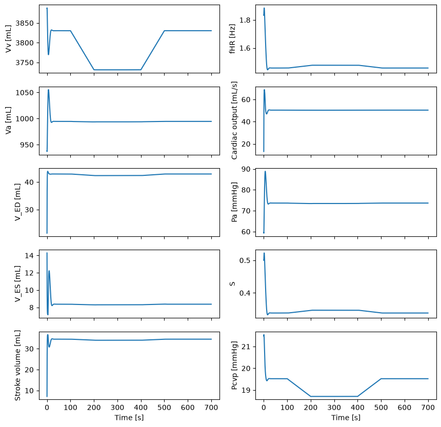
fig, ax = plt.subplots(5, 2, sharex=True, figsize=(10, 10))
ax[0, 0].plot(time, history["Vv"][start_plot:])
ax[0, 0].set_ylabel("Vv [mL]")
ax[1, 0].plot(time, history["Va"][start_plot:])
ax[1, 0].set_ylabel("Va [mL]")
ax[2, 0].plot(time, history["V_ED"][start_plot:])
ax[2, 0].set_ylabel("V_ED [mL]")
ax[3, 0].plot(time, history["V_ES"][start_plot:])
ax[3, 0].set_ylabel("V_ES [mL]")
SV = np.subtract(history["V_ED"], history["V_ES"])
ax[4, 0].plot(time, SV[start_plot:], label="SV")
ax[4, 0].set_ylabel("Stroke volume [mL]")
ax[0, 1].plot(time, history["fHR"][start_plot:])
ax[0, 1].set_ylabel("fHR [Hz]")
CO = SV * history["fHR"]
ax[1, 1].plot(time, CO[start_plot:], label="CO")
ax[1, 1].set_ylabel("Cardiac output [mL/s]")
ax[2, 1].plot(time, history["Pa"][start_plot:])
ax[2, 1].set_ylabel("Pa [mmHg]")
ax[3, 1].plot(time, history["S"][start_plot:])
ax[3, 1].set_ylabel("S")
ax[4, 1].plot(time, history["Pcvp"][start_plot:])
ax[4, 1].set_ylabel("Pcvp [mmHg]")
ax[4, 0].set_xlabel("Time [s]")
ax[4, 1].set_xlabel("Time [s]")
# plt.show()
fig.savefig("zenker.png")
References#
[ZRC19]
Sven Zenker, Jonathan Rubin, and Gilles Clermont. Correction: from inverse problems in mathematical physiology to quantitative differential diagnoses. PLoS Computational Biology, 15(6):e1007155, 2019.