Regazzoni 2020#
In this example we will use the 0D model from [RSA+22] to simulate the cardiac cycle.
from circulation.log import setup_logging
from circulation.regazzoni2020 import Regazzoni2020
import matplotlib.pyplot as plt
setup_logging()
circulation = Regazzoni2020()
[06/29/26 20:15:15] INFO     INFO:circulation.base:                                                                                                                                          base.py:134
                                                    Circulation model parameters (Regazzoni2020)
                             ┏━━━━━━━━━━━━━━━━━━━━━━━━━━━━━━━━━━━━━━━┳━━━━━━━━━━━━━━━━━━━━━━━━━━━━━━━━━━━━━━━━━━━━━━━━━┓
                             ┃ Parameter                             ┃ Value                                           ┃
                             ┡━━━━━━━━━━━━━━━━━━━━━━━━━━━━━━━━━━━━━━━╇━━━━━━━━━━━━━━━━━━━━━━━━━━━━━━━━━━━━━━━━━━━━━━━━━┩
                             │ HR                                    │ 1.25 hertz                                      │
                             │ chambers.LA.EA                        │ 0.07 millimeter_Hg / milliliter                 │
                             │ chambers.LA.EB                        │ 0.18 millimeter_Hg / milliliter                 │
                             │ chambers.LA.TC                        │ 0.17 second                                     │
                             │ chambers.LA.TR                        │ 0.17 second                                     │
                             │ chambers.LA.tC                        │ 0.9 second                                      │
                             │ chambers.LA.V0                        │ 4.0 milliliter                                  │
                             │ chambers.LV.EA                        │ 4.482 millimeter_Hg / milliliter                │
                             │ chambers.LV.EB                        │ 0.17 millimeter_Hg / milliliter                 │
                             │ chambers.LV.TC                        │ 0.25 second                                     │
                             │ chambers.LV.TR                        │ 0.4 second                                      │
                             │ chambers.LV.tC                        │ 0.1 second                                      │
                             │ chambers.LV.V0                        │ 42.0 milliliter                                 │
                             │ chambers.RA.EA                        │ 0.06 millimeter_Hg / milliliter                 │
                             │ chambers.RA.EB                        │ 0.07 millimeter_Hg / milliliter                 │
                             │ chambers.RA.TC                        │ 0.17 second                                     │
                             │ chambers.RA.TR                        │ 0.17 second                                     │
                             │ chambers.RA.tC                        │ 0.9 second                                      │
                             │ chambers.RA.V0                        │ 4.0 milliliter                                  │
                             │ chambers.RV.EA                        │ 0.2 millimeter_Hg / milliliter                  │
                             │ chambers.RV.EB                        │ 0.029 millimeter_Hg / milliliter                │
                             │ chambers.RV.TC                        │ 0.25 second                                     │
                             │ chambers.RV.TR                        │ 0.4 second                                      │
                             │ chambers.RV.tC                        │ 0.1 second                                      │
                             │ chambers.RV.V0                        │ 16.0 milliliter                                 │
                             │ valves.MV.Rmin                        │ 0.0075 millimeter_Hg * second / milliliter      │
                             │ valves.MV.Rmax                        │ 75006.2 millimeter_Hg * second / milliliter     │
                             │ valves.AV.Rmin                        │ 0.0075 millimeter_Hg * second / milliliter      │
                             │ valves.AV.Rmax                        │ 75006.2 millimeter_Hg * second / milliliter     │
                             │ valves.TV.Rmin                        │ 0.0075 millimeter_Hg * second / milliliter      │
                             │ valves.TV.Rmax                        │ 75006.2 millimeter_Hg * second / milliliter     │
                             │ valves.PV.Rmin                        │ 0.0075 millimeter_Hg * second / milliliter      │
                             │ valves.PV.Rmax                        │ 75006.2 millimeter_Hg * second / milliliter     │
                             │ circulation.SYS.R_AR                  │ 0.733 millimeter_Hg * second / milliliter       │
                             │ circulation.SYS.C_AR                  │ 1.372 milliliter / millimeter_Hg                │
                             │ circulation.SYS.R_VEN                 │ 0.32 millimeter_Hg * second / milliliter        │
                             │ circulation.SYS.C_VEN                 │ 11.363 milliliter / millimeter_Hg               │
                             │ circulation.SYS.L_AR                  │ 0.005 millimeter_Hg * second ** 2 / milliliter  │
                             │ circulation.SYS.L_VEN                 │ 0.0005 millimeter_Hg * second ** 2 / milliliter │
                             │ circulation.PUL.R_AR                  │ 0.046 millimeter_Hg * second / milliliter       │
                             │ circulation.PUL.C_AR                  │ 20.0 milliliter / millimeter_Hg                 │
                             │ circulation.PUL.R_VEN                 │ 0.0015 millimeter_Hg * second / milliliter      │
                             │ circulation.PUL.C_VEN                 │ 16.0 milliliter / millimeter_Hg                 │
                             │ circulation.PUL.L_AR                  │ 0.0005 millimeter_Hg * second ** 2 / milliliter │
                             │ circulation.PUL.L_VEN                 │ 0.0005 millimeter_Hg * second ** 2 / milliliter │
                             │ circulation.external.start_withdrawal │ 0.0 second                                      │
                             │ circulation.external.end_withdrawal   │ 0.0 second                                      │
                             │ circulation.external.start_infusion   │ 0.0 second                                      │
                             │ circulation.external.end_infusion     │ 0.0 second                                      │
                             │ circulation.external.flow_withdrawal  │ 0.0 milliliter / second                         │
                             │ circulation.external.flow_infusion    │ 0.0 milliliter / second                         │
                             └───────────────────────────────────────┴─────────────────────────────────────────────────┘
                    INFO     INFO:circulation.base:                                                                                                                                          base.py:141
                                  Circulation model initial states
                                           (Regazzoni2020)
                             ┏━━━━━━━━━━━┳━━━━━━━━━━━━━━━━━━━━━━━━━━━━━┓
                             ┃ State     ┃ Value                       ┃
                             ┡━━━━━━━━━━━╇━━━━━━━━━━━━━━━━━━━━━━━━━━━━━┩
                             │ V_LA      │ 87.183 milliliter           │
                             │ V_LV      │ 118.52 milliliter           │
                             │ V_RA      │ 86.833 milliliter           │
                             │ V_RV      │ 166.177 milliliter          │
                             │ p_AR_SYS  │ 87.675 millimeter_Hg        │
                             │ p_VEN_SYS │ 35.898 millimeter_Hg        │
                             │ p_AR_PUL  │ 19.545 millimeter_Hg        │
                             │ p_VEN_PUL │ 15.004 millimeter_Hg        │
                             │ Q_AR_SYS  │ 71.104 milliliter / second  │
                             │ Q_VEN_SYS │ 94.039 milliliter / second  │
                             │ Q_AR_PUL  │ 94.084 milliliter / second  │
                             │ Q_VEN_PUL │ 473.279 milliliter / second │
                             └───────────┴─────────────────────────────┘
history = circulation.solve(num_beats=10)
circulation.print_info()
                    INFO     INFO:circulation.base:                                                                                                                                          base.py:512
                                                                                        Volumes
                             ┏━━━━━━━━┳━━━━━━━━━┳━━━━━━━━┳━━━━━━━━━┳━━━━━━━━━━┳━━━━━━━━━━━┳━━━━━━━━━━┳━━━━━━━━━━━┳━━━━━━━━━┳━━━━━━━━━┳━━━━━━━━━┳━━━━━━━━━━┓
                             ┃ V_LA   ┃ V_LV    ┃ V_RA   ┃ V_RV    ┃ V_AR_SYS ┃ V_VEN_SYS ┃ V_AR_PUL ┃ V_VEN_PUL ┃ Heart   ┃ SYS     ┃ PUL     ┃ Total    ┃
                             ┡━━━━━━━━╇━━━━━━━━━╇━━━━━━━━╇━━━━━━━━━╇━━━━━━━━━━╇━━━━━━━━━━━╇━━━━━━━━━━╇━━━━━━━━━━━╇━━━━━━━━━╇━━━━━━━━━╇━━━━━━━━━╇━━━━━━━━━━┩
                             │ 87.204 │ 118.659 │ 86.768 │ 166.139 │ 120.380  │ 408.167   │ 390.770  │ 239.789   │ 458.770 │ 528.547 │ 630.559 │ 1617.876 │
                             └────────┴─────────┴────────┴─────────┴──────────┴───────────┴──────────┴───────────┴─────────┴─────────┴─────────┴──────────┘

                                                                 Pressures
                             ┏━━━━━━━━┳━━━━━━━━┳━━━━━━━┳━━━━━━━┳━━━━━━━━━━┳━━━━━━━━━━━┳━━━━━━━━━━┳━━━━━━━━━━━┓
                             ┃ p_LA   ┃ p_LV   ┃ p_RA  ┃ p_RV  ┃ p_AR_SYS ┃ p_VEN_SYS ┃ p_AR_PUL ┃ p_VEN_PUL ┃
                             ┡━━━━━━━━╇━━━━━━━━╇━━━━━━━╇━━━━━━━╇━━━━━━━━━━╇━━━━━━━━━━━╇━━━━━━━━━━╇━━━━━━━━━━━┩
                             │ 14.938 │ 12.988 │ 5.801 │ 4.348 │ 87.740   │ 35.921    │ 19.538   │ 14.987    │
                             └────────┴────────┴───────┴───────┴──────────┴───────────┴──────────┴───────────┘

                                                                     Flows
                             ┏━━━━━━━━━┳━━━━━━━━┳━━━━━━━━━┳━━━━━━━━┳━━━━━━━━━━┳━━━━━━━━━━━┳━━━━━━━━━━┳━━━━━━━━━━━┓
                             ┃ Q_MV    ┃ Q_AV   ┃ Q_TV    ┃ Q_PV   ┃ Q_AR_SYS ┃ Q_VEN_SYS ┃ Q_AR_PUL ┃ Q_VEN_PUL ┃
                             ┡━━━━━━━━━╇━━━━━━━━╇━━━━━━━━━╇━━━━━━━━╇━━━━━━━━━━╇━━━━━━━━━━━╇━━━━━━━━━━╇━━━━━━━━━━━┩
                             │ 257.845 │ -0.001 │ 191.446 │ -0.000 │ 71.163   │ 94.123    │ 94.382   │ 470.060   │
                             └─────────┴────────┴─────────┴────────┴──────────┴───────────┴──────────┴───────────┘
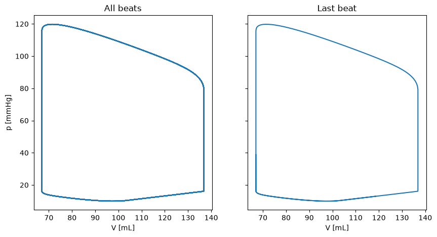
fig, ax = plt.subplots(1, 2, sharex=True, sharey=True, figsize=(10, 5))
ax[0].plot(history["V_LV"], history["p_LV"])
ax[0].set_xlabel("V [mL]")
ax[0].set_ylabel("p [mmHg]")
ax[0].set_title("All beats")
ax[1].plot(history["V_LV"][-1000:], history["p_LV"][-1000:])
ax[1].set_title("Last beat")
ax[1].set_xlabel("V [mL]")
Text(0.5, 0, 'V [mL]')
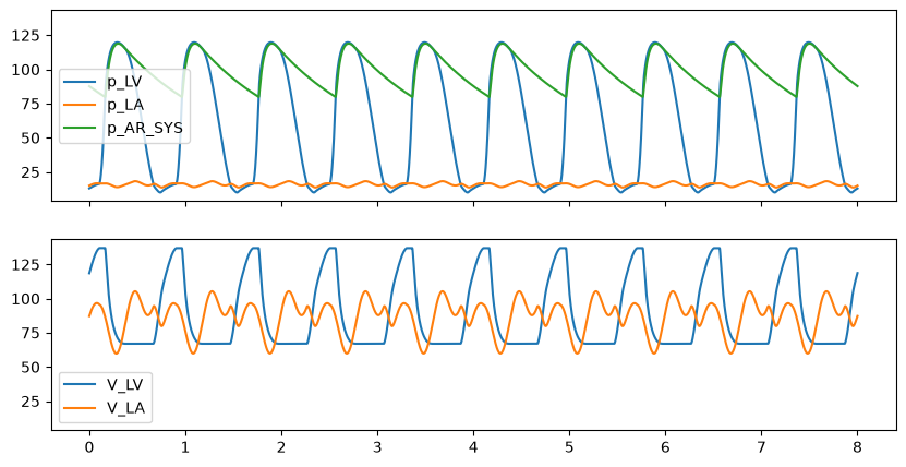
fig, ax = plt.subplots(2, 1, sharex=True, sharey=True, figsize=(10, 5))
ax[0].plot(history["time"], history["p_LV"], label="p_LV")
ax[0].plot(history["time"], history["p_LA"], label="p_LA")
ax[0].plot(history["time"], history["p_AR_SYS"], label="p_AR_SYS")
ax[0].legend()
ax[1].plot(history["time"], history["V_LV"], label="V_LV")
ax[1].plot(history["time"], history["V_LA"], label="V_LA")
ax[1].legend()
<matplotlib.legend.Legend at 0x7f2c641a1250>
plt.show()
References#
[RSA+22]
Francesco Regazzoni, Matteo Salvador, Pasquale Claudio Africa, Marco Fedele, Luca Dedè, and Alfio Quarteroni. A cardiac electromechanical model coupled with a lumped-parameter model for closed-loop blood circulation. Journal of Computational Physics, 457:111083, 2022.