Everything in simcardemsx starts from a single cell model: a system of ordinary differential equations (ODEs) describing one cardiomyocyte. This first tutorial uses no mesh and no finite elements. It runs the cell model on its own, then shows how simcardemsx cuts it in two so that it can be coupled to tissue mechanics.
The cell model
The model used throughout these tutorials joins two published models in one
gotranx .ode file:
Electrophysiology (EP): the ToR-ORd model of a human ventricular myocyte (Tomek et al., eLife 2019), in its dynamic-chloride variant for endocardial cells. It describes the membrane potential , the ion currents that shape the action potential, and the calcium handling that releases calcium into the cytosol ().
Contraction: the Land model of human cardiac muscle (Land et al., J Mol Cell Cardiol 2017). Calcium binds to troponin (
CaTrpn), which frees myosin to form crossbridges. These attach in a weakly bound state (XW) and move to a strongly bound state (XS). Two distortion states (Zetas,Zetaw) follow how far the attached crossbridges are stretched when the fibre lengthens or shortens. The active tension the cell generates iswhere is the stretch of the fibre and its length dependence. Through and the stretch rate (
dLambda), the tension depends on what the tissue is doing. That is what makes the coupling between cell and tissue two-way.
The contraction and EP equations are joined in both directions. Calcium drives the contraction, and the calcium bound to troponin is taken out of the cytosol, which feeds back onto EP. This is mechano-electric feedback.
The repository ships the same cell model in three .ode files, in
examples/odefiles.
They differ only in where the line between EP and mechanics is drawn, which we come
back to below.
from pathlib import Path

import gotranx
import matplotlib.pyplot as plt
import numpy as np

from simcardemsx.ode_model import load_ode_modules

# Run as a script, this is the script's own folder; run as a notebook, the notebook's.
HERE = Path(__file__).resolve().parent if "__file__" in globals() else Path.cwd()
ODEFILES = HERE.parent / "odefiles"
odefile = ODEFILES / "ToRORd_dynCl_endo_zetasplit.ode"
Running the whole cell
gotranx turns an .ode file into Python code. Here we generate the whole model as
plain NumPy, with the generalized Rush-Larsen (GRL) scheme, which takes exponential
steps for the gating variables and so allows a much larger time step than forward
Euler.
ode = gotranx.load_ode(odefile)
code = gotranx.cli.gotran2py.get_code(ode, scheme=[gotranx.schemes.Scheme.generalized_rush_larsen])
cell: dict = {}
exec(code, cell)

print(f"{len(ode.states)} states, {len(ode.parameters)} parameters")
print("components:", ", ".join(sorted(c.name for c in ode.components)))
2026-11-09 14:05:38 [info ] Load ode /__w/simcardemsx/simcardemsx/examples/odefiles/ToRORd_dynCl_endo_zetasplit.ode
2026-11-09 14:05:42 [warning ] Dropping a guard whose replacement failed its numeric check value=0 var=clss
2026-11-09 14:05:42 [warning ] Dropping a guard whose replacement failed its numeric check value=0 var=nai
2026-11-09 14:05:42 [warning ] Dropping a guard whose replacement failed its numeric check value=0 var=ki
2026-11-09 14:05:42 [warning ] Dropping a guard whose replacement failed its numeric check value=0 var=cli
2026-11-09 14:05:43 [info ] Num states 52
2026-11-09 14:05:43 [info ] Num parameters 140
52 states, 140 parameters
components: CaMK, ICaL, ICab, ICl, IK1, IKb, IKr, IKs, INa, INaCa, INaK, INaL, INab, I_katp, IpCa, Ito, SERCA, cell_geometry, diff, environment, extracellular, intracellular_ions, mechanics, mechanics-ep, membrane, physical_constants, reversal_potentials, ryr, trans_flux
The fibre stretch (lmbda) and its rate (dLambda) are parameters of the
cell model. Left at their defaults (, ) the cell
contracts isometrically: it generates tension but cannot shorten. The model’s own
stimulus current fires at and then once every second.
dt = 0.05  # ms
t_end = 1000.0  # ms, one beat
y = cell["init_state_values"]()
p = cell["init_parameter_values"]()
v_i, cai_i = cell["state_index"]("v"), cell["state_index"]("cai")
Ta_i = cell["monitor_index"]("Ta")

times = np.arange(0.0, t_end, dt)
v, cai, Ta = np.zeros_like(times), np.zeros_like(times), np.zeros_like(times)
for n, t in enumerate(times):
    v[n], cai[n] = y[v_i], y[cai_i]
    Ta[n] = cell["monitor_values"](t, y, p)[Ta_i]
    y = cell["generalized_rush_larsen"](y, t, dt, p)
fig, axes = plt.subplots(1, 3, figsize=(12, 3.2), sharex=True)
axes[0].plot(times, v)
axes[0].set(ylabel="v [mV]", title="Action potential")
axes[1].plot(times, cai * 1e3)
axes[1].set(ylabel="[Ca$^{2+}$]$_i$ [µM]", title="Calcium transient")
axes[2].plot(times, Ta)
axes[2].set(ylabel="$T_a$ [kPa]", title="Active tension (isometric)")
for ax in axes:
ax.set_xlabel("time [ms]")
fig.tight_layout()
plt.show()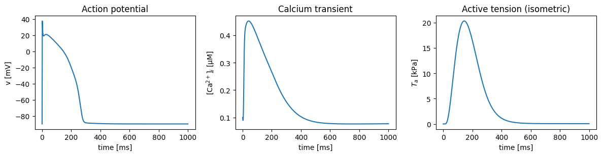
The three traces follow each other. The action potential opens the L-type calcium channels, which triggers calcium release from the sarcoplasmic reticulum. The calcium transient peaks a few tens of milliseconds later, and tension follows more slowly still, peaking well after the calcium has started to fall.
print(f"peak v      {v.max():7.1f} mV at {times[v.argmax()]:6.1f} ms")
print(f"peak cai    {cai.max() * 1e3:7.3f} µM at {times[cai.argmax()]:6.1f} ms")
print(f"peak Ta     {Ta.max():7.2f} kPa at {times[Ta.argmax()]:6.1f} ms")
peak v 37.6 mV at 1.6 ms
peak cai 0.452 µM at 41.1 ms
peak Ta 20.30 kPa at 144.4 ms
Splitting the cell in two
In a tissue simulation the two halves of this model do not live in the same place.
EP is solved by fenicsx-beat. It steps the ODE at every node of the EP mesh with a small time step (0.05 ms here), with a reaction-diffusion equation (the monodomain model) spreading the action potential between the nodes.
Mechanics is solved by fenicsx-pulse, on its own mesh and with a larger time step (1 ms or more). The tension enters the stress at every quadrature point of the mechanics mesh.
Each .ode file therefore marks one component as "mechanics". Those states are
stepped on the mechanics mesh, and everything else is stepped by EP.
simcardemsx.ode_model.load_ode_modules cuts the file along that line and
generates two modules. The EP half is NumPy code for beat. The mechanics half is
UFL, the symbolic form language of FEniCSx, so the mechanics solver can
differentiate through it (tutorial 3 shows why that matters).
Generating ToR-ORd takes about 15 seconds. The code is cached in the output folder and
reused until the .ode file or gotranx changes.
modules = load_ode_modules(odefile, HERE / "generated_odes" / odefile.stem)

print("EP module:        ", len(modules.ep.state), "states")
print("mechanics module: ", len(modules.mechanics.state), "states:", list(modules.mechanics.state))
EP module: 49 states
mechanics module: 3 states: ['Zetaw', 'Zetas', 'Cd']
Each generated module records, as plain dictionaries, what it needs from the other
side (missing) and what it hands over (provides). In this split, the mechanics
side holds only the two distortion states and Cd. To compute the tension it needs
XS and XW from EP, and EP in turn needs Zetas and Zetaw back from mechanics.
print("mechanics needs   ", modules.mechanics.missing)
print("EP provides       ", modules.ep.provides)
print("EP needs          ", modules.ep.missing)
print("mechanics provides", modules.mechanics.provides)
mechanics needs {'XS': 0, 'XW': 1}
EP provides {'XS': 0, 'XW': 1}
EP needs {'Zetas': 0, 'Zetaw': 1}
mechanics provides {'Zetas': 0, 'Zetaw': 1}
The fibre stretch is the other quantity that crosses back. It is not produced by
the ODE at all but by the mechanics solve, so it crosses as the EP parameter lmbda,
if EP has one.
print("lmbda is an EP parameter:", "lmbda" in modules.ep.parameter)lmbda is an EP parameter: True
The three splits
The same cell can be cut in different places. The further the cut is moved towards EP, the more of the contraction model is stepped on the mechanics mesh, and the fewer variables have to cross.
print(f"{'split':12s} {'EP states':>9s} {'mech states':>11s}  EP → mechanics      mechanics → EP")
for split in ("zetasplit", "catrpnsplit", "caisplit"):
    path = ODEFILES / f"ToRORd_dynCl_endo_{split}.ode"
    m = load_ode_modules(path, HERE / "generated_odes" / path.stem)
    back = list(getattr(m.ep, "missing", {}))
    if "lmbda" in m.ep.parameter:
        back.append("lmbda")
    print(
        f"{split:12s} {len(m.ep.state):9d} {len(m.mechanics.state):11d}  "
        f"{', '.join(m.mechanics.missing):18s}  {', '.join(back) or '-'}",
    )
split EP states mech states EP → mechanics mechanics → EP
zetasplit 49 3 XS, XW Zetas, Zetaw, lmbda
2026-11-09 14:06:06 [info ] Load ode /__w/simcardemsx/simcardemsx/examples/odefiles/ToRORd_dynCl_endo_catrpnsplit.ode
2026-11-09 14:06:11 [warning ] Dropping a guard whose replacement failed its numeric check value=0 var=clss
2026-11-09 14:06:11 [warning ] Dropping a guard whose replacement failed its numeric check value=0 var=nai
2026-11-09 14:06:11 [warning ] Dropping a guard whose replacement failed its numeric check value=0 var=ki
2026-11-09 14:06:11 [warning ] Dropping a guard whose replacement failed its numeric check value=0 var=cli
2026-11-09 14:06:11 [info ] Num states 52
2026-11-09 14:06:11 [info ] Num parameters 145
catrpnsplit         46           6  CaTrpn              lmbda
caisplit            45           7  cai                 J_TRPN
zeta split: only the distortion states are on the mechanics side. The crossbridge populations come from EP.
CaTrpn split: the whole Land model except troponin binding is on the mechanics side. Only
CaTrpncrosses, and nothing comes back.Ca split: the whole Land model is on the mechanics side. It receives the cytosolic calcium and returns the troponin buffering flux
J_TRPNto EP.
Whatever is on the mechanics side lives at the quadrature points of the mechanics mesh. The stretch it sees there is the true fibre stretch of the deforming tissue, not an average carried over from EP. The next tutorial shows why it matters how that stretch is fed into the contraction model.