The first tutorial showed that the active tension depends on the fibre stretch and on the stretch rate . In a coupled simulation comes from the mechanics solve, and the mechanics solve needs the tension. Something has to decide, at every time step, which comes first.
The obvious answer is to take turns. Step the contraction model with the stretch of the last step, then solve mechanics with the resulting tension held fixed. This is a segregated (staggered) scheme. It lets each physics keep its own solver, mesh and time step.
It also fails, in a way that is easy to mistake for a solver problem.
Regazzoni & Quarteroni (CMAME 2021) showed that this scheme’s amplification factor tends to as . Here is the active stiffness of the tissue and the passive one. Once , which is routine in contracting myocardium, the factor is below -1. The scheme is then not merely inaccurate but not convergent, and refining the time step makes it worse.
This tutorial reproduces their Test Case 1 in 0D, so it runs in seconds and needs no mesh. It compares three ways of coupling the same contraction model to the same tissue:
monolithic: contraction and mechanics solved together. This is the reference.
segregated: the naive staggered scheme.
stabilized: segregated, plus one consistent extra term.
The fix is small. Instead of treating the active tension as a dead load during the mechanics solve, treat it as what it physically is, crossbridges behaving as springs:
Here is the stretch of the last step, the deformation gradient and the fibre direction. The added term is and vanishes in the limit, so it does not change the problem being solved. It only makes the scheme stable.
import matplotlib.pyplot as plt
import numpy as np

from simcardemsx import zero_d
Setting up
The tissue is R&Q’s 0D model, a single fibre whose strain balances
in the quasistatic regime they analyse (). The contraction model is Land’s (2017), as in tutorial 1, here from the crossbridge package.
The passive stiffness Kp is the knob that decides everything. With a stiff tissue the
naive scheme is fine, and with a soft one it is not. We run both.
simcardemsx.zero_d works in seconds and pascals, following the paper. The rest of
simcardemsx uses milliseconds.
soft = zero_d.Tissue(Kp=2e4, M=0.0, sigma=0.0)  # Ka will exceed Kp
stiff = zero_d.Tissue(Kp=1e6, M=0.0, sigma=0.0)  # Ka stays below Kp

T_END = 0.4  # s
DT = 1e-3  # s
The drive is R&Q’s Eq. (57), an idealised calcium transient peaking at 1.6 µM.
t = np.linspace(0, T_END, 400)
fig, ax = plt.subplots(figsize=(6, 2.4))
ax.plot(t, zero_d.calcium_transient(t), color="#12706B")
ax.set(xlabel="time [s]", ylabel="[Ca$^{2+}$]$_i$ [µM]", title="Stimulus")
fig.tight_layout()
plt.show()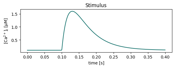
The stable case
With a stiff tissue, all three schemes agree. Nothing here suggests a problem, which is the trap.
stable = zero_d.compare(tissue=stiff, dt=DT, T=T_END)
for scheme in zero_d.SCHEMES:
    err = stable.error_against_monolithic(scheme)
    ratio = stable[scheme].Ka.max() / stiff.Kp
    print(f"{scheme:12s} peak Ka/Kp = {ratio:5.2f}   error = {err:.2e}")
monolithic peak Ka/Kp = 0.17 error = 0.00e+00
segregated peak Ka/Kp = 0.17 error = 3.64e-06
stabilized peak Ka/Kp = 0.17 error = 3.76e-06
The unstable case
Soften the tissue so that the active stiffness overtakes the passive stiffness during the twitch, and the naive scheme comes apart.
unstable = zero_d.compare(tissue=soft, dt=DT, T=T_END)
for scheme in zero_d.SCHEMES:
    r = unstable[scheme]
    ratio = r.Ka.max() / soft.Kp
    print(f"{scheme:12s} peak Ka/Kp = {ratio:5.2f}   oscillation = {r.oscillation_metric:.3f}")
monolithic peak Ka/Kp = 5.73 oscillation = 0.008
segregated peak Ka/Kp = 5.32 oscillation = 0.263
stabilized peak Ka/Kp = 5.88 oscillation = 0.008
STYLE = {
    "monolithic": dict(color="#16191C", lw=2.4, label="monolithic (reference)"),
    "segregated": dict(color="#B33F0C", lw=1.2, label="segregated (naive)"),
    "stabilized": dict(color="#12706B", lw=1.6, ls="--", label="stabilized"),
}

fig, axes = plt.subplots(2, 2, figsize=(11, 6), sharex=True)
for col, (name, comparison) in enumerate(
    [("stiff tissue: $K_a < K_p$", stable), ("soft tissue: $K_a > K_p$", unstable)],
):
    for scheme in zero_d.SCHEMES:
        r = comparison[scheme]
        axes[0, col].plot(r.t, r.Ta / 1000.0, **STYLE[scheme])
        axes[1, col].plot(r.t, r.stretch, **STYLE[scheme])
    axes[0, col].set_title(name)
    axes[1, col].set_xlabel("time [s]")

axes[0, 0].set_ylabel("active tension [kPa]")
axes[1, 0].set_ylabel("fibre stretch $\\lambda$ [-]")
axes[0, 1].legend(frameon=False, fontsize=9)
fig.tight_layout()
plt.show()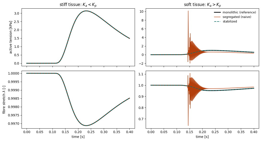
The right-hand column is the point. The naive scheme oscillates from one step to the next, while the stabilized one tracks the monolithic reference closely enough to be hard to tell apart from it.
Refinement does not save the naive scheme
This is what makes the instability worth understanding rather than just avoiding. A scheme that is merely inaccurate gets better as the time step is refined. This one does not.
print(f"{'dt':>8} | {'naive osc':>10} {'naive err':>10} | {'stab osc':>9} {'stab err':>10}")
errors: dict[str, list[float]] = {"segregated": [], "stabilized": []}
dts = [4e-3, 2e-3, 1e-3, 5e-4]
for dt in dts:
    c = zero_d.compare(tissue=soft, dt=dt, T=T_END)
    for name in errors:
        errors[name].append(c.error_against_monolithic(name))
    print(
        f"{dt:8.0e} | {c['segregated'].oscillation_metric:10.3f} {errors['segregated'][-1]:10.2e} "
        f"| {c['stabilized'].oscillation_metric:9.3f} {errors['stabilized'][-1]:10.2e}",
    )
dt | naive osc naive err | stab osc stab err
   4e-03 |      0.313   2.59e-01 |     0.030   3.16e-03
   2e-03 |      0.276   3.51e-01 |     0.015   1.62e-03
1e-03 | 0.263 3.53e-01 | 0.008 8.18e-04
/dolfinx-env/lib/python3.12/site-packages/simcardemsx/zero_d.py:69: RuntimeWarning: invalid value encountered in log1p
  return 0.5 * self.Kp * (np.log1p(e) + e / (1.0 + e))
5e-04 | 0.661 nan | 0.004 4.11e-04
fig, ax = plt.subplots(figsize=(5.5, 4))
for scheme in ("segregated", "stabilized"):
    ax.loglog(dts, errors[scheme], "o-", color=STYLE[scheme]["color"], label=STYLE[scheme]["label"])
ax.loglog(dts, np.array(dts) * errors["stabilized"][0] / dts[0], "k:", lw=1, label="first order")
ax.set(xlabel="$\\Delta t$ [s]", ylabel="max strain error vs monolithic")
ax.legend(frameon=False)
ax.invert_xaxis()
fig.tight_layout()
plt.show()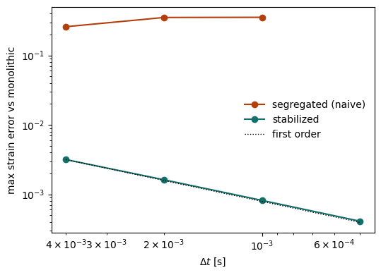
The stabilized scheme converges at first order, as its consistency argument says it
should. The naive one does not converge, and its error grows as the step shrinks:
there is no time step small enough to fix it. At the smallest step the naive run breaks
down altogether. Its strain passes -1, where the tissue’s energy is undefined (the
RuntimeWarning above), so its error prints as nan and is missing from the plot.
What this means in practice
Any contraction model that responds to shortening velocity will do this when coupled naively to a soft enough tissue, and that is most of them, since the response is what produces the force-velocity relationship. The symptom is a solution that oscillates at the time-step frequency, which is easy to misread as a Newton tolerance problem or a mesh problem.
simcardemsx offers two ways out, and both are used in the next tutorial.
Monolithic:
GeneratedActivation(..., scheme="monolithic"), the default, steps the contraction model inside the mechanics Newton iteration. The model is generated as UFL from the.odefile, so Newton differentiates through it. This needs no extra term, but it needs a model that can be written in UFL.Stabilized:
GeneratedActivation(..., scheme="stabilized"), orCrossbridgeSegregatedfor the NumPy models of the crossbridge package, which cannot be stepped inside Newton. Its stabilization is on by default:from simcardemsx.backends import CrossbridgeSegregated backend = CrossbridgeSegregated(f0, mesh, "Land2017", quadrature_degree=4)
scheme="segregated" and stabilized=False exist only to reproduce the failure shown
above.