The previous tutorials took the pieces apart. This one puts them together: an action potential spreads across a small slab of tissue, the calcium it releases makes the tissue contract, and the contraction feeds back into the electrophysiology.
Two solvers, each on its own mesh and with its own time step, are coupled:
EP: the monodomain model, solved by fenicsx-beat with operator splitting. The ODE step advances the EP half of the cell model at every node, and the PDE step diffuses the membrane potential :
Here is the membrane surface-to-volume ratio, the membrane capacitance, the (anisotropic) conductivity tensor and the cell model’s states.
Mechanics: quasistatic, solved by fenicsx-pulse, with the contraction half of the cell model stepped inside Newton by
GeneratedActivation, as in tutorial 3.
simcardemsx.controller.SimulationController runs the coupled loop. Every mechanics
step of it
runs EP steps;
sends what the contraction model needs from EP to the mechanics mesh;
solves mechanics and accepts the step (
begin_step, solve,post_solve);sends what EP needs back (here the distortion states and the stretch ), averaged onto the EP mesh.
What crosses is not configured by hand. It is read off the generated modules’
missing and provides dictionaries, which tutorial 1 printed. If a step fails, the
controller restores every component to where it was before the step and raises.
import time
from pathlib import Path

from mpi4py import MPI

import beat
import dolfinx
import matplotlib.pyplot as plt
import numpy as np
import pulse

from simcardemsx.backends import GeneratedActivation
from simcardemsx.controller import SimulationController
from simcardemsx.ode_model import load_ode_modules
from simcardemsx.transfer_plan import resolve

HERE = Path(__file__).resolve().parent if "__file__" in globals() else Path.cwd()
odefile = HERE.parent / "odefiles" / "ToRORd_dynCl_endo_zetasplit.ode"
modules = load_ode_modules(odefile, HERE / "generated_odes" / odefile.stem)
2026-11-09 14:03:20 [info ] Load ode /__w/simcardemsx/simcardemsx/examples/odefiles/ToRORd_dynCl_endo_zetasplit.ode
2026-11-09 14:03:25 [warning ] Dropping a guard whose replacement failed its numeric check value=0 var=ki
2026-11-09 14:03:25 [warning ] Dropping a guard whose replacement failed its numeric check value=0 var=nai
2026-11-09 14:03:25 [warning ] Dropping a guard whose replacement failed its numeric check value=0 var=cli
2026-11-09 14:03:25 [warning ] Dropping a guard whose replacement failed its numeric check value=0 var=clss
2026-11-09 14:03:25 [info ] Num states 52
2026-11-09 14:03:25 [info ] Num parameters 140
The slab
A 3 × 1 × 0.5 mm slab with fibres along . EP and mechanics share this mesh here. They need not: the transfer between them interpolates between any two meshes.
LX, LY, LZ, DX = 3.0, 1.0, 0.5, 0.25  # mm
mesh = dolfinx.mesh.create_box(
    MPI.COMM_WORLD,
    [[0.0, 0.0, 0.0], [LX, LY, LZ]],
    [round(LX / DX), round(LY / DX), round(LZ / DX)],
    dolfinx.mesh.CellType.tetrahedron,
)
f0 = dolfinx.fem.Constant(mesh, np.array([1.0, 0.0, 0.0]))
s0 = dolfinx.fem.Constant(mesh, np.array([0.0, 1.0, 0.0]))
print(f"{mesh.topology.index_map(3).size_global} cells")
576 cells
Electrophysiology
The cell model’s own stimulus current is switched off (i_Stim_Amplitude = 0).
Instead a stimulus current is applied for 2 ms in the corner mm, from
where the action potential spreads through the slab.
DT_EP = 0.05  # ms
chi = beat.units.ureg.Quantity(140.0, "mm**-1")
C_m = beat.units.ureg.Quantity(0.01, "uF/mm**2")

M = beat.conductivities.define_conductivity_tensor(
    chi=chi,
    f0=f0,
    g_il=0.17 * beat.units.ureg("S/m"),
    g_it=0.019 * beat.units.ureg("S/m"),
    g_el=0.62 * beat.units.ureg("S/m"),
    g_et=0.24 * beat.units.ureg("S/m"),
)

corner = dolfinx.mesh.locate_entities(
    mesh,
    3,
    lambda x: (x[0] <= 0.5 + 1e-6) & (x[1] <= 0.5 + 1e-6) & (x[2] <= 0.5 + 1e-6),
)
stim_tags = dolfinx.mesh.meshtags(mesh, 3, corner, np.full(corner.size, 1, dtype=np.int32))

time_ep = dolfinx.fem.Constant(mesh, 0.0)
I_s = beat.stimulation.define_stimulus(
    mesh=mesh,
    chi=chi,
    time=time_ep,
    subdomain_data=stim_tags,
    marker=1,
    mesh_unit="mm",
    amplitude=50_000.0 * beat.units.ureg("uA/cm**3"),
    start=0.0,
    duration=2.0,
)
pde = beat.MonodomainModel(
    time=time_ep,
    mesh=mesh,
    M=M,
    I_s=I_s,
    C_m=C_m.to("uF/mm**2").magnitude,
)
The ODE is stepped at every node of a P1 space. States, parameters and the variables coming from mechanics are stored with one column per node. The controller writes the stretch and the distortion states into these arrays in place, and they differ from node to node.
ep_module = modules.ep
V_ode = dolfinx.fem.functionspace(mesh, ("P", 1))
v_ode = dolfinx.fem.Function(V_ode)
num_points = v_ode.x.array.size

states = np.tile(ep_module.init_state_values()[:, None], (1, num_points))
parameters = np.tile(
    ep_module.init_parameter_values(i_Stim_Amplitude=0.0)[:, None],
    (1, num_points),
)
ode = beat.odesolver.DolfinODESolver(
    v_ode=v_ode,
    v_pde=pde.state,
    fun=ep_module.generalized_rush_larsen,
    init_states=states,
    parameters=parameters,
    num_states=len(states),
    v_index=ep_module.state_index("v"),
    missing_variables=np.zeros((len(ep_module.missing), num_points)),
    num_missing_variables=len(ep_module.missing),
)
ep_solver = beat.MonodomainSplittingSolver(pde=pde, ode=ode, theta=1)Mechanics
This is the problem of tutorial 3 on the slab, with rollers on the three faces through the origin. The displacement is P2, and the contraction states live at the quadrature points of a degree 4 rule, which must match the form’s.
QUADRATURE_DEGREE = 4

backend = GeneratedActivation(
    modules.mechanics,
    mesh,
    f0,
    quadrature_degree=QUADRATURE_DEGREE,
    scheme="monolithic",
)
model = pulse.CardiacModel(
    material=pulse.HolzapfelOgden(
        f0=f0,
        s0=s0,
        **pulse.HolzapfelOgden.transversely_isotropic_parameters(),
    ),
    active=backend,
    compressibility=pulse.Incompressible(),
)


def rollers(V):
    """u_i = 0 on the face x_i = 0, for i = 0, 1, 2."""
    V0, _ = V.sub(0).collapse()
    zero = dolfinx.fem.Function(V0)
    bcs = []
    for i in range(3):
        facets = dolfinx.mesh.locate_entities_boundary(
            mesh,
            2,
            lambda x, i=i: np.isclose(x[i], 0.0),
        )
        dofs = dolfinx.fem.locate_dofs_topological((V.sub(i), V0), 2, facets)
        bcs.append(dolfinx.fem.dirichletbc(zero, dofs, V.sub(i)))
    return bcs


petsc_options = pulse.StaticProblem.default_parameters()["petsc_options"]
petsc_options["snes_atol"] = 1e-9
problem = pulse.StaticProblem(
    model=model,
    geometry=pulse.Geometry(mesh=mesh, metadata={"quadrature_degree": QUADRATURE_DEGREE}),
    bcs=pulse.BoundaryConditions(dirichlet=[rollers]),
    parameters={
        "base_bc": pulse.problem.BaseBC.free,
        "petsc_options": petsc_options,
        "u_space": "P_2",
    },
)Coupling
The controller checks the set-up when it is built: the backend must be the problem’s
active model, a whole multiple of , and the backend’s
quadrature degree the form’s. It then works out what crosses between the two sides,
with simcardemsx.transfer_plan.resolve, which we can call ourselves to see the
answer. It raises if either side needs something the other does not provide.
DT_MECH = 1.0  # ms
controller = SimulationController(
    mechanics=problem,
    ep_solver=ep_solver,
    backend=backend,
    ode_modules=modules,
    dt_mech=DT_MECH,
    dt_ep=DT_EP,
)
crossings = resolve(modules.ep, backend)
print("EP → mechanics:", crossings.forward)
print("mechanics → EP:", crossings.backward)
print("λ sent to EP:  ", crossings.stretch_to_ep)
EP → mechanics: ('XS', 'XW')
mechanics → EP: ('Zetas', 'Zetaw')
λ sent to EP: True
Running
controller.step() advances everything by one mechanics step. Its callbacks are
called after every EP step and after every mechanics step. We use the EP callback to
record when each node is activated (when first rises above 0 mV), and the
mechanics callback to record the means of , and .
T_END = 200.0  # ms
v_index = ep_module.state_index("v")
activation = np.full(num_points, np.nan)
trace: dict[str, list[float]] = {
    "t": [0.0],
    "v": [states[v_index].mean()],
    "lmbda": [1.0],
    "Ta": [0.0],
    "shortening": [0.0],
}


def on_ep_step(t, ep_step):
    v = ep_solver.ode.full_values[v_index]
    newly = np.isnan(activation) & (v > 0.0)
    activation[newly] = t


def on_mech_step(t, mech_step, newton_iterations):
    trace["t"].append(t)
    trace["v"].append(ep_solver.ode.full_values[v_index].mean())
    trace["lmbda"].append(backend.lmbda_prev.x.array.mean())
    trace["Ta"].append(backend.tension_kPa.x.array.mean())
    # The x component of the displacement; the far end moves towards x = 0.
    u_x = problem.u.x.array.reshape(-1, 3)[:, 0]
    trace["shortening"].append(-u_x.min())


start = time.perf_counter()
while controller.t < T_END - 1e-9:
    controller.step(ep_callback=on_ep_step, mech_callback=on_mech_step)
print(f"{T_END:g} ms in {time.perf_counter() - start:.0f} s")
200 ms in 64 s
The activation wave
The activation times on the face show the wave leaving the stimulated corner. It travels faster along the fibres () than across them, because the conductivity is higher along the fibres.
coordinates = V_ode.tabulate_dof_coordinates()
bottom = np.isclose(coordinates[:, 2], 0.0)
fig, ax = plt.subplots(figsize=(7, 2.8))
contours = ax.tricontourf(
    coordinates[bottom, 0],
    coordinates[bottom, 1],
    activation[bottom],
    levels=20,
    cmap="viridis",
)
fig.colorbar(contours, ax=ax, label="activation time [ms]")
ax.set(xlabel="x [mm]", ylabel="y [mm]", aspect="equal", title="Activation times at z = 0")
fig.tight_layout()
plt.show()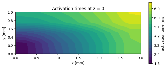
along_x = bottom & np.isclose(coordinates[:, 1], 0.0) & (coordinates[:, 0] >= 1.0)
slope = np.polyfit(coordinates[along_x, 0], activation[along_x], 1)[0]
print(f"conduction velocity along the fibres: {1.0 / slope:.2f} mm/ms = {100.0 / slope:.0f} cm/s")
conduction velocity along the fibres: 0.59 mm/ms = 59 cm/s
Contraction
Tension builds up over the 150 ms after the action potential, as in tutorial 1, and the slab shortens along its fibres.
t = np.array(trace["t"])
fig, axes = plt.subplots(1, 4, figsize=(15, 3.2))
axes[0].plot(t, trace["v"])
axes[0].set(ylabel="mean v [mV]", title="Membrane potential")
axes[1].plot(t, trace["Ta"])
axes[1].set(ylabel="mean $T_a$ [kPa]", title="Active tension")
axes[2].plot(t, trace["lmbda"])
axes[2].set(ylabel="mean $\\lambda$ [-]", title="Fibre stretch")
axes[3].plot(t, np.array(trace["shortening"]) * 1e3)
axes[3].set(ylabel="shortening [µm]", title=f"Shortening of the {LX:g} mm slab")
for ax in axes:
    ax.set_xlabel("time [ms]")
fig.tight_layout()
plt.show()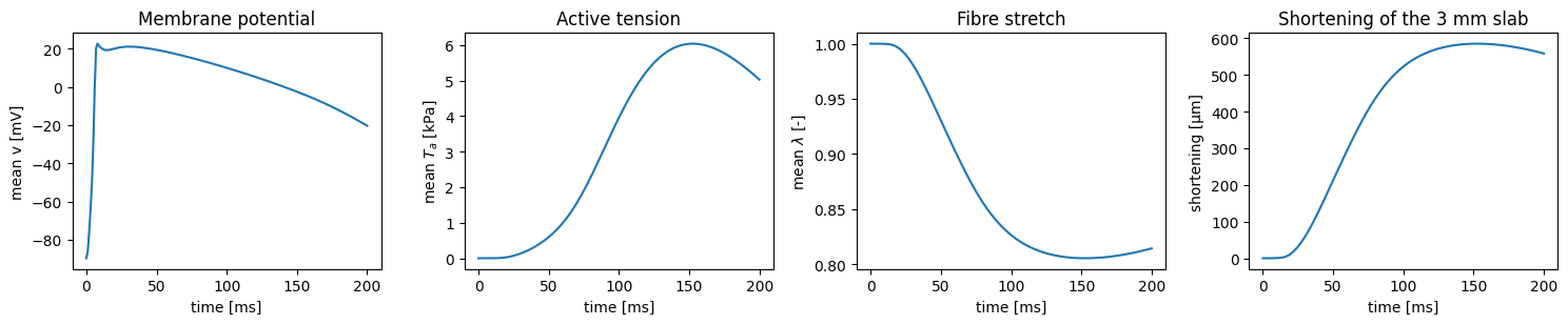
The stretch goes back to EP after every mechanics step, where it enters the
contraction half of the cell model that EP steps. In this split that is the crossbridge
populations XS and XW and troponin binding. This is the mechano-electric feedback of
the model.
lmbda_row = ep_module.parameter_index("lmbda")
lmbda_ep = ode.parameters[lmbda_row]
print(f"λ at the EP nodes after {T_END:g} ms: {lmbda_ep.min():.4f} to {lmbda_ep.max():.4f}")
λ at the EP nodes after 200 ms: 0.8099 to 0.8178
Where to go from here
The slab example is this tutorial grown into a full program. It takes the split, the scheme and a crossbridge model on the command line, writes
results.bpfor ParaView, and checkpoints and restarts.controller.snapshot()andcontroller.restore(snapshot)copy and restore the state of every component, andsimcardemsx.checkpoint.Checkpointerwrites it to disk, so a run can continue in a new process.The BiV and Rodero examples put the same coupling into a beating biventricular heart, closed by a circulation model.