The previous tutorial showed in 0D why the coupling scheme matters. This one does the same with finite elements: a single element of tissue, contracting under a prescribed calcium transient. There is no EP solver yet. The calcium is written straight into the contraction model, so the focus is on the coupling between contraction and mechanics alone.
The pieces are:
a mechanics problem from fenicsx-pulse: a hyperelastic, incompressible material with fibres along ;
an activation backend,
simcardemsx.backends.GeneratedActivation, which owns the contraction model’s states and turns them into an active stress.
The model
The tissue is a Holzapfel-Ogden material (Holzapfel & Ogden, 2009), with strain energy of the right Cauchy-Green tensor . The active tension of the cell model is added along the fibres. simcardemsx uses the normalization of Regazzoni & Quarteroni, under which whatever the stretch:
with the pressure that keeps the tissue incompressible (). The element is held on three faces by rollers and is otherwise free, so it shortens along the fibre when it contracts.
We use the Ca split from tutorial 1, where the whole Land model is on the
mechanics side and its only input is the cytosolic calcium cai.
from pathlib import Path

from mpi4py import MPI

import dolfinx
import matplotlib.pyplot as plt
import numpy as np
import pulse

from simcardemsx.backends import GeneratedActivation
from simcardemsx.ode_model import load_ode_modules

HERE = Path(__file__).resolve().parent if "__file__" in globals() else Path.cwd()
odefile = HERE.parent / "odefiles" / "ToRORd_dynCl_endo_caisplit.ode"
modules = load_ode_modules(odefile, HERE / "generated_odes" / odefile.stem)
print("the backend needs", modules.mechanics.missing, "and provides", modules.mechanics.provides)
2026-11-09 14:04:50 [info ] Load ode /__w/simcardemsx/simcardemsx/examples/odefiles/ToRORd_dynCl_endo_caisplit.ode
2026-11-09 14:04:55 [warning ] Dropping a guard whose replacement failed its numeric check value=0 var=nai
2026-11-09 14:04:55 [warning ] Dropping a guard whose replacement failed its numeric check value=0 var=ki
2026-11-09 14:04:55 [warning ] Dropping a guard whose replacement failed its numeric check value=0 var=clss
2026-11-09 14:04:55 [warning ] Dropping a guard whose replacement failed its numeric check value=0 var=cli
2026-11-09 14:04:55 [info ] Num states 52
2026-11-09 14:04:55 [info ] Num parameters 140
the backend needs {'cai': 0} and provides {'J_TRPN': 0}
The mechanics problem
build returns a pulse.StaticProblem (quasistatic, so no inertia) and the backend
it uses as its active model. The backend’s states live at the quadrature points of the
mechanics form, so its quadrature_degree must be the form’s.
The absolute Newton tolerance snes_atol is tightened from pulse’s default. At rest the
first residual is already at round-off, which a purely relative tolerance cannot
reduce further.
QUADRATURE_DEGREE = 2


def rollers(V):
    """u_i = 0 on the face x_i = 0, for i = 0, 1, 2."""
    mesh = V.mesh
    V0, _ = V.sub(0).collapse()
    zero = dolfinx.fem.Function(V0)
    bcs = []
    for i in range(3):
        facets = dolfinx.mesh.locate_entities_boundary(
            mesh,
            mesh.topology.dim - 1,
            lambda x, i=i: np.isclose(x[i], 0.0),
        )
        dofs = dolfinx.fem.locate_dofs_topological((V.sub(i), V0), mesh.topology.dim - 1, facets)
        bcs.append(dolfinx.fem.dirichletbc(zero, dofs, V.sub(i)))
    return bcs


def build(scheme):
    mesh = dolfinx.mesh.create_unit_cube(MPI.COMM_WORLD, 1, 1, 1)
    f0 = dolfinx.fem.Constant(mesh, np.array([1.0, 0.0, 0.0]))
    s0 = dolfinx.fem.Constant(mesh, np.array([0.0, 1.0, 0.0]))

    backend = GeneratedActivation(
        modules.mechanics,
        mesh,
        f0,
        quadrature_degree=QUADRATURE_DEGREE,
        scheme=scheme,
    )
    model = pulse.CardiacModel(
        material=pulse.HolzapfelOgden(
            f0=f0,
            s0=s0,
            **pulse.HolzapfelOgden.transversely_isotropic_parameters(),
        ),
        active=backend,
        compressibility=pulse.Incompressible(),
    )
    petsc_options = pulse.StaticProblem.default_parameters()["petsc_options"]
    petsc_options["snes_atol"] = 1e-9
    problem = pulse.StaticProblem(
        model=model,
        geometry=pulse.Geometry(mesh=mesh, metadata={"quadrature_degree": QUADRATURE_DEGREE}),
        bcs=pulse.BoundaryConditions(dirichlet=[rollers]),
        parameters={"base_bc": pulse.problem.BaseBC.free, "petsc_options": petsc_options},
    )
    return problem, backend
The time loop
Each mechanics step follows the same protocol, which tutorial 4’s controller also follows:
write the inputs at the new time into
backend.inputs, here a prescribed calcium transient peaking at 1 µM;backend.begin_step(t_n, dt)tells the backend which step is being taken;problem.solve()runs Newton, which assembles the backend’s active stress;backend.post_solve()accepts the step: the contraction states, the stretch and the tension of the converged solution become the new “previous” values.
Nothing is accepted before post_solve, so a step whose Newton solve fails leaves the
backend as it was.
def calcium(t):
    """Ca_i in mM: 0.1 µM at rest, peaking at 1 µM at t = 25 ms."""
    tau = max(t - 5.0, 0.0)
    return 1e-4 + 9e-4 * (tau / 20.0) * np.exp(1.0 - tau / 20.0)


def run(scheme, dt=1.0, t_end=60.0):
    problem, backend = build(scheme)
    times, lmbda, Ta = [0.0], [1.0], [0.0]
    for n in range(round(t_end / dt)):
        t_n, t_next = n * dt, (n + 1) * dt
        backend.inputs["cai"].x.array[:] = calcium(t_next)
        backend.begin_step(t_n, dt)
        if not problem.solve(raise_on_failure=False):
            print(f"{scheme}: Newton failed at t = {t_next} ms")
            break
        backend.post_solve()
        times.append(t_next)
        lmbda.append(backend.lmbda_prev.x.array.mean())
        Ta.append(backend.tension_kPa.x.array.mean())
    return np.array(times), np.array(lmbda), np.array(Ta)


results = {scheme: run(scheme) for scheme in ("monolithic", "stabilized", "segregated")}
Newton did not converge after 9 iterations (SNES converged reason -9)
segregated: Newton failed at t = 31.0 ms
STYLE = {
    "monolithic": dict(color="#16191C", lw=2.4, label="monolithic"),
    "stabilized": dict(color="#12706B", lw=1.6, ls="--", label="stabilized"),
    "segregated": dict(color="#B33F0C", lw=1.0, label="segregated (naive)"),
}
fig, axes = plt.subplots(1, 3, figsize=(13, 3.4))
t = np.linspace(0, 60, 300)
axes[0].plot(t, [calcium(s) * 1e3 for s in t], color="#12706B")
axes[0].set(ylabel="[Ca$^{2+}$]$_i$ [µM]", title="Prescribed calcium")
for scheme, (times, lmbda, Ta) in results.items():
    axes[1].plot(times, Ta, **STYLE[scheme])
    axes[2].plot(times, lmbda, **STYLE[scheme])
# The naive run's spikes would flatten everything else, so the axes are clipped.
axes[1].set(ylabel="$T_a$ [kPa]", title="Active tension", ylim=(-0.5, 4.0))
axes[2].set(ylabel="$\\lambda$ [-]", title="Fibre stretch", ylim=(0.85, 1.05))
axes[2].legend(frameon=False)
for ax in axes:
    ax.set_xlabel("time [ms]")
fig.tight_layout()
plt.show()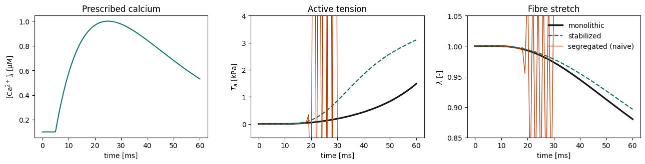
for scheme, (times, lmbda, Ta) in results.items():
    print(
        f"{scheme:11s} reached {times[-1]:5.1f} ms, min stretch {lmbda.min():.4f}, "
        f"peak Ta {Ta.max():6.3f} kPa",
    )
monolithic reached 60.0 ms, min stretch 0.8800, peak Ta 1.482 kPa
stabilized reached 60.0 ms, min stretch 0.8962, peak Ta 3.103 kPa
segregated reached 30.0 ms, min stretch 0.7377, peak Ta 30.006 kPa
The passive material is soft enough here that the active stiffness exceeds the passive one during the twitch, which is the regime of tutorial 2. As in 0D, the naive segregated scheme oscillates from one step to the next from about 20 ms on, until Newton gives up. The other two shorten the element smoothly as the tension rises.
They do not agree with each other at this time step, though. The stabilized scheme adds a term of order , so it is consistent: it converges to the same solution, but at a time step of 1 ms its error is visible. To see both converge, we compare them with a monolithic run at = 0.1 ms, at every whole millisecond.
reference = run("monolithic", dt=0.1)


def at_whole_ms(result, dt):
    times, lmbda, Ta = result
    every = round(1.0 / dt)
    return lmbda[::every], Ta[::every]


lmbda_ref, Ta_ref = at_whole_ms(reference, 0.1)
dts = [1.0, 0.5, 0.25]
errors: dict[str, list[float]] = {"monolithic": [], "stabilized": []}
print(f"{'dt [ms]':>8} {'monolithic':>12} {'stabilized':>12}   (max |λ - λ_ref|)")
for dt in dts:
    for scheme in errors:
        lmbda, _ = at_whole_ms(run(scheme, dt=dt), dt)
        errors[scheme].append(float(np.abs(lmbda - lmbda_ref).max()))
    print(f"{dt:8.2f} {errors['monolithic'][-1]:12.2e} {errors['stabilized'][-1]:12.2e}")
dt [ms] monolithic stabilized (max |λ - λ_ref|)
1.00 4.41e-03 2.01e-02
0.50 1.92e-03 1.10e-02
0.25 7.13e-04 5.66e-03
fig, ax = plt.subplots(figsize=(5.5, 4))
for scheme, err in errors.items():
    ax.loglog(dts, err, "o-", color=STYLE[scheme]["color"], label=STYLE[scheme]["label"])
ax.loglog(dts, np.array(dts) * errors["stabilized"][0] / dts[0], "k:", lw=1, label="first order")
ax.set(xlabel="$\\Delta t$ [ms]", ylabel="max $|\\lambda - \\lambda_{ref}|$")
ax.legend(frameon=False)
ax.invert_xaxis()
fig.tight_layout()
plt.show()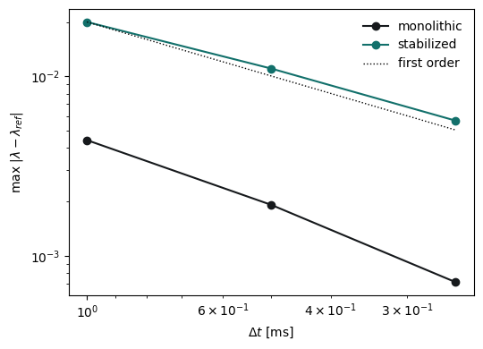
Both converge, at about first order. The stabilized scheme’s error is several times larger at every time step, which is the price of solving the contraction model outside Newton. The monolithic scheme is therefore the default whenever the model can be generated as UFL. The stabilized scheme is the way to couple a model that cannot be.
What the backend computes
GeneratedActivation is a pulse.ActiveModel, so pulse calls its S(C) when it
builds the stress. Under scheme="monolithic", the backend takes one generalized
Rush-Larsen step of the contraction model inside that expression. The step starts from
the last accepted states, with
where is the displacement Newton is currently iterating on. The tension is therefore a UFL function of the displacement, and Newton linearizes through the whole contraction model. That is why the monolithic scheme needs no stabilization.
Besides the stress, the backend exposes a few dolfinx.fem.Functions, written by
post_solve:
| attribute | what it holds |
|---|---|
inputs | what it needs from EP, by name (cai here) |
outputs | what it gives back to EP (J_TRPN here, and lmbda) |
lmbda_prev | the fibre stretch of the last accepted step |
tension_kPa | at the quadrature points, in kPa |
stiffness_kPa | the active stiffness , in kPa |
active_tension | averaged onto P1, for plotting |
The active stiffness is the quantity tutorial 2 compared with the passive one.
problem, backend = build("monolithic")
for n in range(30):
    backend.inputs["cai"].x.array[:] = calcium(n + 1.0)
    backend.begin_step(float(n), 1.0)
    problem.solve()
    backend.post_solve()
print(f"at t = 30 ms: Ta = {backend.tension_kPa.x.array.mean():.3f} kPa")
print(f"              Ka = {backend.stiffness_kPa.x.array.mean():.1f} kPa per unit stretch")
print(f"              J_TRPN = {backend.outputs['J_TRPN'].x.array.mean():.3e} mM/ms")
at t = 30 ms: Ta = 0.192 kPa
Ka = 343.1 kPa per unit stretch
J_TRPN = -1.140e-04 mM/ms
In a full simulation inputs is filled from the EP solver and outputs is sent back
to it. The next tutorial hands that bookkeeping to
SimulationController.