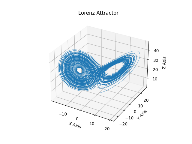
Lorentz Attractor

In this demo we solve the Lorentz attractor

\[\begin{split}\frac{dx}{dt} &= \sigma (y - x) \\ \frac{dy}{dt} &= x (\rho - z) - y \\ \frac{dz}{dt} &= x y - \beta z\end{split}\]

with the parameters \(\sigma=10.0, \rho=28.0\) and \(beta=8/3\) and the initial conditions \(x = 0.0, y = 1.0\), and \(z = 1.05\).

We assume that the we have file called lorentz.ode with the following content

# lorentz.ode
parameters(
sigma=12.0,
rho=21.0,
beta=2.4
)

states(
x=1.0,
y=2.0,
z=3.05
)

dx_dt = sigma * (y - x)
dy_dt = x * (rho - z) - y
dz_dt = x * y - beta * z

And we note that the parameters and initial states are not the same as stated about, so we need to somehow provide the correct parameters and initial states.

First let’s do the usual imports

import goss
import matplotlib.pyplot as plt
import numpy as np
from gotran import load_ode

And load the ode using gotran

lorentz = load_ode("lorentz.ode")

Next we jit-compile the ODE into goss

ode = goss.ParameterizedODE(lorentz)

We can update the parameters using the set_parameter method

ode.set_parameter("sigma", 10.0)
ode.set_parameter("rho", 28.0)
ode.set_parameter("beta", 8 / 3)

We can now instantiate the solver and select the time steps

solver = goss.solvers.RKF32(ode)
t = np.linspace(0, 100, 10001)

We can also provide the correct initial states to the solver

ic = np.array([0.0, 1.0, 1.05])
u = solver.solve(t, y0=ic)

Finally we plot the solution

fig = plt.figure()
ax = fig.add_subplot(projection="3d")
ax.plot(u[:, 0], u[:, 1], u[:, 2], lw=0.5)
ax.set_xlabel("X Axis")
ax.set_ylabel("Y Axis")
ax.set_zlabel("Z Axis")
ax.set_title("Lorenz Attractor")
plt.show()

Fig. 1 Computed solution of the lorentz attractor