Field parameters

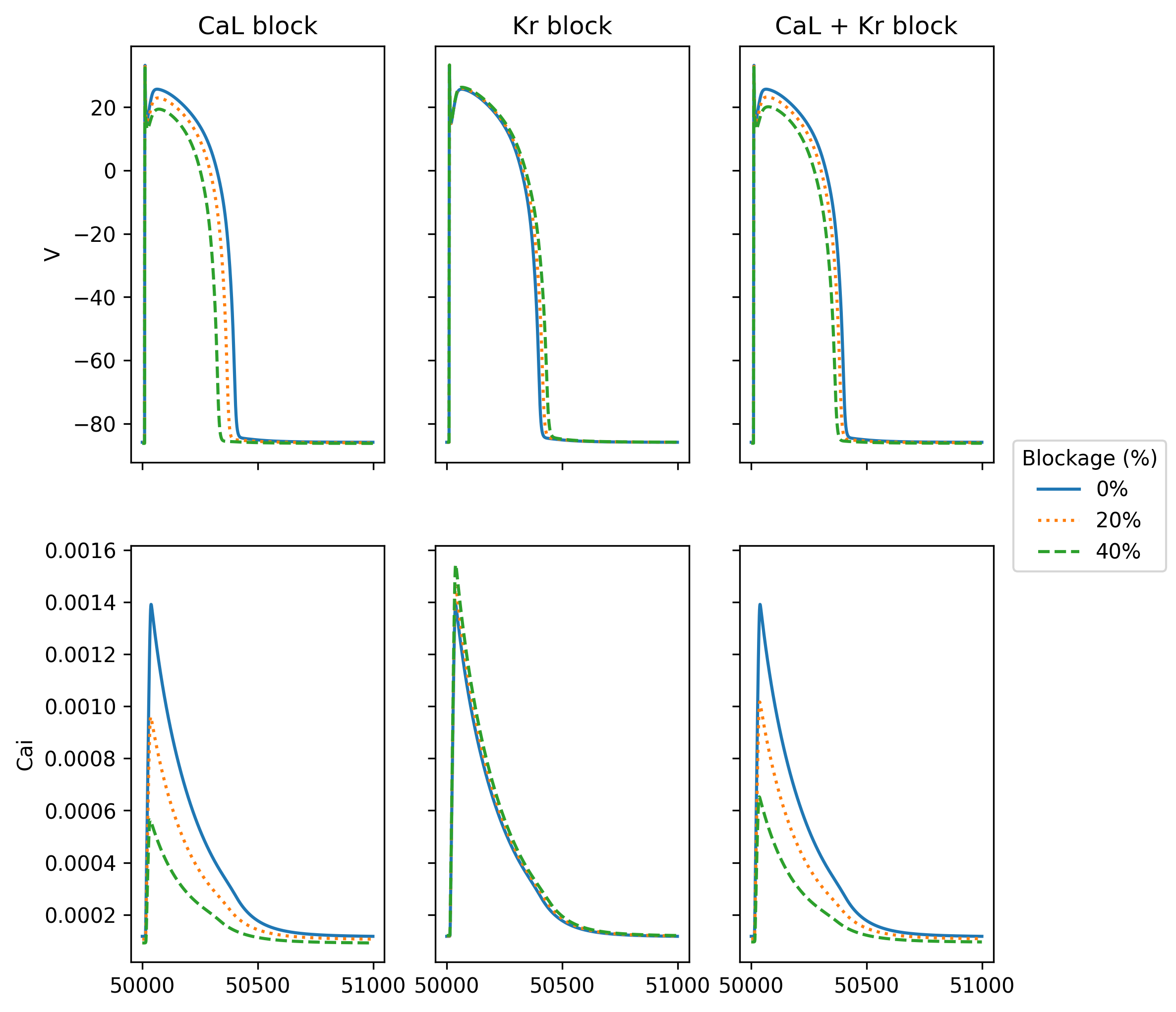
In this demo we will solve the Tentusscher mode [TTP06] for a number of different parameters in the model. More specifically, we would like to simulate a drug that blocks one or two channels in the cells. We will block the CaL- and the Kr-channel with 0%, 20% and 40% and we would like to do this both with CaL alone, Kr alone and a combined block. In other words, we would like to run 9 different simulations where the only differrence is the value of these parameters.

First we need to make the necessary imports

import time

import goss
import matplotlib.pyplot as plt
import numpy as np
from gotran import load_ode

We select the field parameters to be g_CaL and g_Kr which are the conductances of the channels Scaling these parameters will simulate the effect of a drug targeting these channels

field_parameters = ["g_CaL", "g_Kr"]

We would also like to keep track of the membrane potential (V) and the intracellular calcium concentrations for each of the parameter sets, and we therefore specify these states as fields states

field_state_names = ["V", "Ca_i"]

We supply these additional arguments to the ParameterizedODE class

ode = goss.ParameterizedODE(
    load_ode("tentusscher_panfilov_2006_M_cell.ode"),
    field_states=field_state_names,
    field_parameters=field_parameters,
)

We use the first order generalized rush larsen scheme and set an internal step size of 0.01

solver = goss.solvers.GRL1()
solver.internal_time_step = 0.01

We will run 9 different parameter sets so we set the number of nodes to 9 and instantiate the ODESystemSolver

num_nodes = 9
system = goss.ODESystemSolver(num_nodes, solver, ode)

Let us also set the number of threads to 9 in order to run each parameter set in parallel

system.num_threads = 9

Now, let us pick three block factors (1 representing baseline)

block_factors = np.array([1, 0.8, 0.6])

and update the field parameters

field_parameters = system.field_parameters
# Block only CaL
field_parameters[:3, 0] *= block_factors
# Block only Kr
field_parameters[3:6, 1] *= block_factors
# Block both
field_parameters[6:9, 0] *= block_factors
field_parameters[6:9, 1] *= block_factors

Note that the field parameters array has dimension number of nodes \(\times\) number of field parameters. In the first three nodes we update only g_CaL which has index 0, while for the nodes 3 to 6 we update g_Kr which has index 1. Finally we need tp update the field parameters on the system solver

system.field_parameters = field_parameters

Let us fist run the forward model for 50 000 ms

T = 50_000
t0 = time.perf_counter()
system.forward(0, T)

And the run it for 1000 ms where we keep track of the field states

tstop = 1000.0
dt = 1.0
time_stamps = np.arange(T, T + tstop, dt)
field_states = system.solve(time_stamps)
print(f"Elapsed time: {time.perf_counter() - t0}")

Finally let us plot the resulting field states for each parameter set

lines = []
labels = []
fig, ax = plt.subplots(2, 3, figsize=(8, 8), sharex=True, sharey="row")
for i, color in enumerate(["g", "b", "r"]):
    for j, linestyle in enumerate(["-", ":", "--"]):
        (l,) = ax[0, i].plot(
            time_stamps,
            field_states[:, 3 * i + j, 0],
            linestyle=linestyle,
        )
        ax[1, i].plot(
            time_stamps,
            field_states[:, 3 * i + j, 1],
            linestyle=linestyle,
        )
        if i == 0:
            labels.append(f"{round((1-block_factors[j])*100)}%")
            lines.append(l)

ax[0, 0].set_title("CaL block")
ax[0, 1].set_title("Kr block")
ax[0, 2].set_title("CaL + Kr block")
ax[0, 0].set_ylabel("V")
ax[1, 0].set_ylabel("Cai")
lgd = fig.legend(lines, labels, title="Blockage (%)", loc="center right")
fig.subplots_adjust(right=0.85)
fig.savefig(
    "tentusscher_field_parameters.png",
    bbox_extra_artists=(lgd,),
    bbox_inches="tight",
    dpi=300,
)
plt.show()

Fig. 6 Computed solution of the membrane potential (V) and the intracellular calcium concentration in the Tentusscher model for different blockage of CaL and Kr

References

[TTP06]

Kirsten HWJ Ten Tusscher and Alexander V Panfilov. Alternans and spiral breakup in a human ventricular tissue model. American Journal of Physiology-Heart and Circulatory Physiology, 291(3):H1088–H1100, 2006.