Solving ODEs on a mesh

In this demo we will demonstrate how you can solve an ODE for each point in the mesh, where the mesh is defined in FEniCS. This might be relevant if you want to solve an ODE for different parameter sets, where the parameters have some spatial dependence. While this example is somewhat artificial it demonstrates how you could do this.

First we make the necessary imports

import gotran
import dolfin
import goss
import numpy as np
import matplotlib.pyplot as plt

We will use the Loretnz attractor model as an example

ode = gotran.load_ode("lorentz.ode")

And we will use thr RKF32 solver and 12 threads.

params = goss.dolfinutils.DOLFINODESystemSolver.default_parameters()
params["num_threads"] = 12
params["solver"] = "RKF32"

We will solve this one a UnitSquare mesh with 3x3 elements, and we will keep track of the \(y\)-coordinate. We will also select beta as a field parameter which will be a spatially resolved parameter

mesh = dolfin.UnitSquareMesh(3, 3)
ode = goss.dolfinutils.DOLFINParameterizedODE(
    ode,
    field_states=["y"],
    field_parameters=["beta"],
)

We let beta be a parameter in \(\mathbb{P}1\) with an expression that depeds on the \(y\)-coordinate

V_beta = dolfin.FunctionSpace(mesh, "Lagrange", 1)
beta = dolfin.Function(V_beta)
beta.interpolate(dolfin.Expression("2.4*x[1] + 0.2", degree=1))
ode.set_parameter("beta", beta)

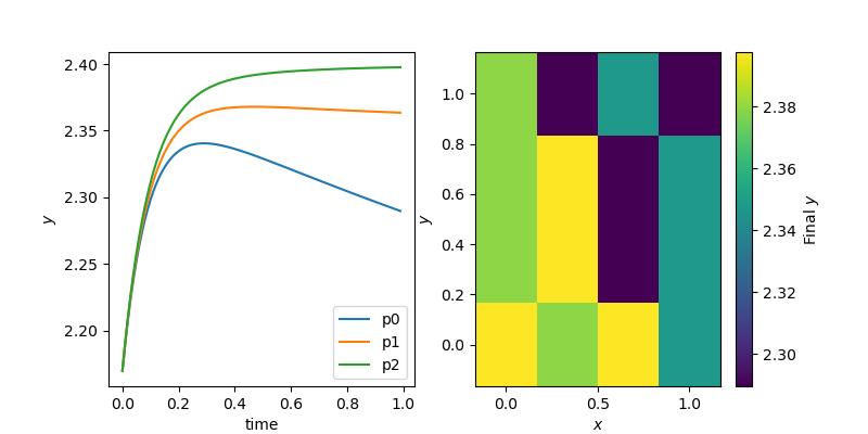
We select three different points that we will track just to see what the solution of \(y\) looks like in these points.

p0 = (0.0, 0.0)
p1 = (0.5, 0.5)
p2 = (1.0, 1.0)

We also print out the value of the beta at these three points

print("Beta at p0: ", beta(p0))
print("Beta at p1: ", beta(p1))
print("Beta at p2: ", beta(p2))

Now we create the system solver, and let our field states be in a \(\mathbb{P}1\) space as well

ode_solver = goss.dolfinutils.DOLFINODESystemSolver(
    mesh,
    odes=ode,
    params=params,
    space="P_1",
)

We all keep track of the solution

vs = ode_solver.vs

Now we make the time stepping. We will simulate this for 1.0 second with a time step of 0.1. At each step we evaluate the solution at the three predefined points and store the solution

dt = 0.01
T = 1.0
time = np.arange(0, T, dt)
solutions = np.empty((3, len(time)))
t = 0.0
for i, t in enumerate(time):
    ode_solver.step((t, t + dt))
    solutions[0, i] = vs(p0)
    solutions[1, i] = vs(p1)
    solutions[2, i] = vs(p2)

# We can also prepare a heatmap showing the final $y$ values for different point in the mesh
coords = vs.function_space().tabulate_dof_coordinates()
x = np.unique(coords[:, 0])
y = np.unique(coords[:, 1])
X, Y = np.meshgrid(x, y)
Z = vs.vector().get_local().reshape((len(y), len(x)))

# Finally let us plot the traces of the selected points and the heat map
fig, ax = plt.subplots(1, 2, figsize=(8, 4))
ax[0].plot(time, solutions[0, :], label="p0")
ax[0].plot(time, solutions[1, :], label="p1")
ax[0].plot(time, solutions[2, :], label="p2")
ax[0].set_ylabel("$y$")
ax[0].set_xlabel("time")
ax[0].legend()
im = ax[1].pcolormesh(X, Y, Z)
cbar = fig.colorbar(im, ax=ax[1])
cbar.set_label("Final $y$")
ax[1].set_xlabel("$x$")
ax[1].set_ylabel("$y$")
fig.savefig("odes_on_mesh.png")

Fig. 7 To the left we show the time course of the \(y\) coordinate of three selected points. To the right we see the final \(y\) coordinate at each point in the mesh.