Tentusscher model#
In this demo we will solve the Tentusscher mode [TTP06]. This is a stiff set of ODEs modeling the action potential in cardiac cells. Since this is a stiff system we would need to make some adjustments in order to be able to solve the system
First we need to make the necessary imports
import goss
import matplotlib.pyplot as plt
import numpy as np
from gotran import load_ode
And load the ode
gotran_ode = load_ode("tentusscher_panfilov_2006_M_cell.ode")
ode = goss.ParameterizedODE(gotran_ode)
One thing we could to is to use a simple solver, e.g the Explicit Euler scheme, but you will soon realize that you need to pick a large number of time steps in order to make this converge.
solver = goss.solvers.ExplicitEuler(ode)
In stead of selecting a large number of time steps, you can instead set a low internal step
solver.internal_time_step = 0.001
This will ensure that for each time step there are additional time steps. However, we will instead use an adaptive implicit solver which is much better suited for these kinds of ODEs. The particular solver we use here is the ESDIRK23a, which is an explicit singly diagonal implicit Runge-Kutta method with an advancing method of order 2 and error estimator of order 3.
solver = goss.solvers.ESDIRK23a(ode)
We select some time steps and solve the system
dt = 1.0
T = 1000
t = np.arange(0, 1000 + dt, dt)
y = solver.solve(t)
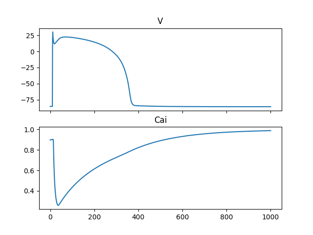
We also grab the indices of the membrane potential (V) and the intracellular calcium concentration
V_index = gotran_ode.state_symbols.index("V")
Cai_index = gotran_ode.state_symbols.index("Ca_i")
and plot these solutions
fig, ax = plt.subplots(2, 1, sharex=True)
ax[0].plot(t, y[:, V_index])
ax[1].plot(t, y[:, Cai_index])
ax[0].set_title("V")
ax[1].set_title("Cai")
fig.savefig("tentusscher.png")
plt.show()

Fig. 5 Computed solution of the membrane potential (V) and the intracellular calcium concentration in the Tentusscher model#
References#
Kirsten HWJ Ten Tusscher and Alexander V Panfilov. Alternans and spiral breakup in a human ventricular tissue model. American Journal of Physiology-Heart and Circulatory Physiology, 291(3):H1088–H1100, 2006.
