Oscilator - Using the forward method

In this demo we will solve a simple oscilator ODE by calling the forward method on the ODE-solver. All ODE-solvers implements this method and the difference between the different solvers lies in how this method is implemented.

First we need to make the necessary imports

import goss
import matplotlib.pyplot as plt
import numpy as np
from gotran import load_ode

The first we need to do is to write the ODE-file. This ODE has the form

\[\begin{split}\frac{dx}{dt} &= -y \\ \frac{dy}{dt} &= x\end{split}\]

with the initial conditions \(x = 1.0\) and \(y = 0.0\). We can writes this in a gotran ode file as follows

# oscilator.ode
states(x=1.0, y=0.)

dx_dt = -y
dy_dt = x

Note that the df_dt syntax, where f is a state is a special syntax in gotran that indicates the derivative.

Next we load the ODE file using gotran and supply this to the goss.ODE class constructor.

oscilator = goss.ODE(load_ode("oscilator.ode"))

This will create the C++ code and jit compile it using cppyy. Next we need to pick a solver (you can use the cli goss list-solvers to see all options). Here we pick the simplest possible solver, the explicit Euler scheme.

solver = goss.solvers.ExplicitEuler(oscilator)

Now we select the time steps

tstop = 10.0
n_steps = 1000
time = np.linspace(0, tstop, n_steps + 1)
dt = time[1] - time[0]

We also keep track of the exact solution of the ODE

u_exact = np.array([np.cos(time), np.sin(time)])

We initialize the arrays for the state

u0 = np.array([1.0, 0.0])
u = np.zeros_like(u_exact)
u[:, 0] = u0

And we make a for loop in python that calls the forward method.

ui = u0
for step in range(1, n_steps + 1):
    t = time[step]
    solver.forward(ui, t, dt)
    u[:, step] = ui

Note that this approach is very slow and should be avoided is you only want to simply solve the whole ode in one go. This method is attractive if you only want to call out to the forward method, for example as a part of a bigger system where you need to solve a system of ODEs at each time step (for example when solving the Monodomain or Bidomains equations (TODO: Add demo about this))

If you only want to solve the ODE (like in this case), you should instead you the solve method

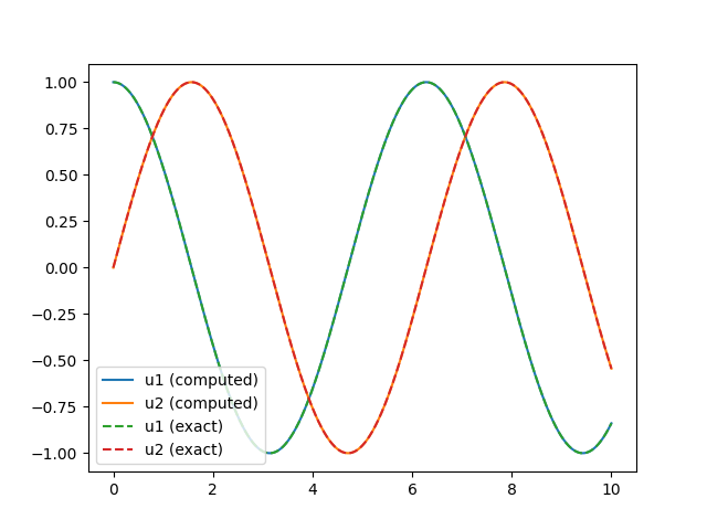
Finally you can plot the solution.

fig, ax = plt.subplots()
ax.plot(time, u[0, :], label="u1 (computed)")
ax.plot(time, u[1, :], label="u2 (computed)")
ax.plot(time, u_exact[0, :], label="u1 (exact)", linestyle="--")
ax.plot(time, u_exact[1, :], label="u2 (exact)", linestyle="--")
ax.legend()
plt.show()

Fig. 2 Computed and exact solution of the oscilator ODE.