Oscilator - Using the solve method

In this demo we will solve a simple oscilator ODE by calling the solve method on the ODE-solver. This a wrapper around the forward method that will solve the ODE for multiple timesteps.

First we need to make the necessary imports

import goss
import matplotlib.pyplot as plt
import numpy as np
from gotran import load_ode

The first we need to do is to write the ODE-file. This ODE has the form

\[\begin{split}\frac{dx}{dt} &= -y \\ \frac{dy}{dt} &= x\end{split}\]

with the initial conditions \(x = 1.0\) and \(y = 0.0\). We can writes this in a gotran ode file as follows

# oscilator.ode
states(x=1.0, y=0.)

dx_dt = -y
dy_dt = x

Note that the df_dt syntax, where f is a state is a special syntax in gotran that indicates the derivative.

Next we load the ODE file using gotran and supply this to the goss.ODE class constructor.

oscilator = goss.ParameterizedODE(load_ode("oscilator.ode"))

This will create the C++ code and jit compile it using cppyy. Next we need to pick a solver (you can use the cli goss list-solvers to see all options). Here we pick the first order Rush-Larsen scheme.

solver = goss.solvers.RL1(oscilator)

Now we select the time steps we want to use and

dt = 0.01
t = np.arange(0, 10 + dt, dt)

We also get the initial conditions from the ODE

u0 = oscilator.get_ic()

And we provide the time steps and the initial conditions to the solve method. Note that we didn’t really need to specify the initial conditions here because if these are not provided then the default initial conditions will be used.

u = solver.solve(t, y0=u0)

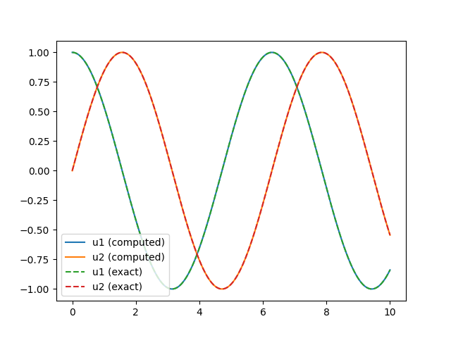
Finally we plot the computed solutions agains the exact solution

u_exact = np.array([np.cos(t), np.sin(t)])
fig, ax = plt.subplots()
ax.plot(t, u[:, 0], label="u1 (computed)")
ax.plot(t, u[:, 1], label="u2 (computed)")
ax.plot(t, u_exact[0, :], label="u1 (exact)", linestyle="--")
ax.plot(t, u_exact[1, :], label="u2 (exact)", linestyle="--")
ax.legend()
plt.show()

Fig. 3 Computed and exact solution of the oscilator ODE.