Custom stimulus domain

In this example we will show how to apply the stimulus to a custom domain. By default the stimulus is applied to the entire EP mesh, but it might be of interest to stimulate only a small region in order to generate a traveling wave and to study features such as conduction velocity.

First me make the necessary imports

from pathlib import Path
import dolfin
import matplotlib.pyplot as plt
import simcardems
import numpy as np

And we specify the path to the output directory where we want to store the results

here = Path(__file__).absolute().parent
outdir = here / "results_custom_stimulus_domain"

There are two way to specify the stimulus domain. One way is to define function which takes as input the EP mesh and outputs an instance of simcardems.geometry.StimulusDomain. This object is basically just a tuple containing the domain (i.e a dolfin.MeshFunction with markers for the domain), and a marker (i.e an integer) representing the value for where the stimulus should be applied.

In this case, we are using a slab geometry of dimensions \([0, 5] \times [0, 2] \times [0, 1] \subset \mathbb{R}^3\), and we will mark the regions were \(x < 1.0\) as the stimulus domain

def stimulus_domain(mesh):
    marker = 1
    subdomain = dolfin.CompiledSubDomain("x[0] < 1.0")
    domain = dolfin.MeshFunction("size_t", mesh, mesh.topology().dim())
    domain.set_all(0)
    subdomain.mark(domain, marker)
    return simcardems.geometry.StimulusDomain(domain=domain, marker=marker)

The other approach is to simply provide the instance of StimulusDomain directly, but this means that you need to have the EP mesh available, which might not always be the case. The benefit of just supply a function is that we might want to perform mesh refinements of the EP mesh in which case a function that can be applied after the mesh refinement is attractable.

Let’s go ahead and load the geometry and also supple the argument for the stimulus_domain

geo = simcardems.geometry.load_geometry(
    mesh_path="geometries/slab.h5",
    stimulus_domain=stimulus_domain,
)

We create the configurations

config = simcardems.Config(
    outdir=outdir,
    coupling_type="fully_coupled_ORdmm_Land",
    T=1000,
)

And create the coupling. Note that, here we are using a different method than usual for creating the coupling, since we need to also supply the geometry.

coupling = simcardems.models.em_model.setup_EM_model_from_config(
    config=config,
    geometry=geo,
)

Next we create the runner, and solve the problem

runner = simcardems.Runner.from_models(config=config, coupling=coupling)
runner.solve(T=config.T, save_freq=config.save_freq, show_progress_bar=True)

Now let us only extract the results of the membrane potential, and compare the values in different points in the mesh. For the slab geometry we can for example evaluate the functions a the minimum and maximum \(x\) values and at the center. To do this, we need to first load the results

loader = simcardems.DataLoader(outdir / "results.h5")

And then extract the relevant traces. Here we also provide a list of names, that contains a tuple of the group and name that we want to extract, e.g the name "V" from the group "ep".

xmin_values = simcardems.postprocess.extract_traces(
    loader,
    reduction="xmin",
    names=[("ep", "V")],
)
xmax_values = simcardems.postprocess.extract_traces(
    loader,
    reduction="xmax",
    names=[("ep", "V")],
)
center_values = simcardems.postprocess.extract_traces(
    loader,
    reduction="center",
    names=[("ep", "V")],
)

Now let us plot these traces in two subplots, were we zoom in at the upstroke in the first subplots

fig, ax = plt.subplots(1, 2, figsize=(8, 4), sharey=True)
ax[0].plot(loader.time_stamps, xmin_values["ep"]["V"], label="xmin")
ax[0].plot(loader.time_stamps, xmax_values["ep"]["V"], label="xmax")
ax[0].plot(loader.time_stamps, center_values["ep"]["V"], label="center")
ax[0].legend()
ax[0].set_ylabel("Voltage [mV]")
ax[0].set_xlabel("Time [ms]")
ax[0].set_xlim(0, 100)
ax[0].set_xticks(np.arange(0, 100, 20))
ax[1].plot(loader.time_stamps, xmin_values["ep"]["V"], label="xmin")
ax[1].plot(loader.time_stamps, xmax_values["ep"]["V"], label="xmax")
ax[1].plot(loader.time_stamps, center_values["ep"]["V"], label="center")
ax[1].legend()
ax[1].set_xlabel("Time [ms]")
ax[1].set_xticks(np.arange(0, 1100, 200))
fig.savefig(outdir / "voltage.png")

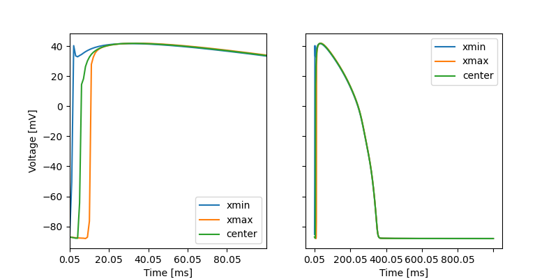
Fig. 10 The membrane potential evaluated at three different points, with a stimulus domain at \(x < 1\). Left subplot shows a zoom in at the upstroke.

It might also be interesting to look at the activation map and display the time it takes for the voltage to reach some threshold value.

To do this we will first create an iterator the we can loop through and give us the next voltage function from the results

time_stamps = loader.time_stamps or []

def voltage_traces():
    for t in time_stamps:
        yield loader.get("ep", "V", t)

Next we use a function for computing the activation map, and indicate that the threshold value should be 0.0. The activation map, will then be a function over the mesh where the value at a given point will be the time it takes for the voltage to first reach 0.0 mV.

activation_map = simcardems.postprocess.activation_map(
    voltage_traces(),
    time_stamps=time_stamps,
    V=loader._functions["ep"]["V"].function_space(),
    threshold=0.0,
)

We can visualize this function in paraview

with dolfin.XDMFFile((outdir / "activation_map.xdmf").as_posix()) as xdmf:
    xdmf.write(activation_map)

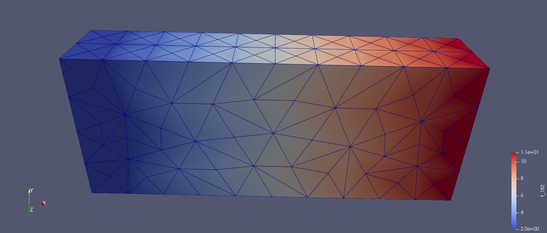
Fig. 11 Activation map of all nodes in the mesh

We can also compute the activation times for all points through the center of the mesh, from \(x=0\) to \(x=L_x\).

x = np.linspace(0, geo.parameters["lx"], 50)
act = [activation_map(xi, geo.parameters["ly"] / 2, geo.parameters["lz"] / 2) for xi in x]
fig, ax = plt.subplots()
ax.plot(x, act)
ax.set_xlabel("$x$ coordinate")
ax.set_ylabel("Activation time [ms]")
ax.grid()
fig.savefig(outdir / "activation_times.png")

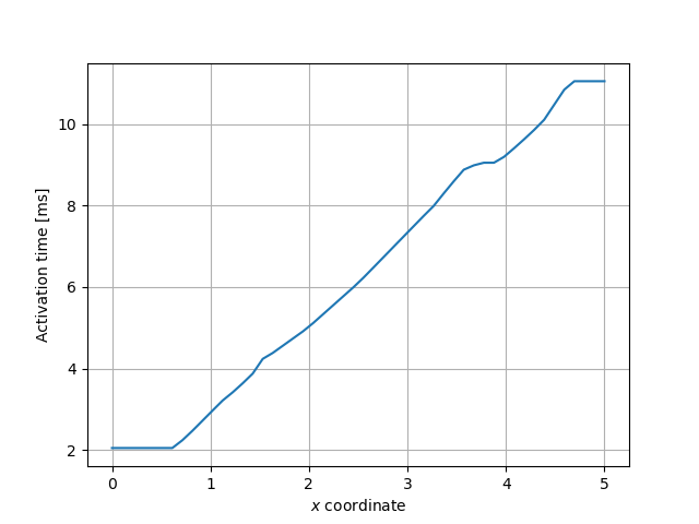
Fig. 12 Activation times through the center of the mesh.