Niederer benchmark

In this example we will use the same setup as in the Niederer benchmark

Niederer SA, Kerfoot E, Benson AP, Bernabeu MO, Bernus O, Bradley C, Cherry EM, Clayton R, Fenton FH, Garny A, Heidenreich E, Land S, Maleckar M, Pathmanathan P, Plank G, Rodríguez JF, Roy I, Sachse FB, Seemann G, Skavhaug O, Smith NP. Verification of cardiac tissue electrophysiology simulators using an N-version benchmark. Philos Trans A Math Phys Eng Sci. 2011 Nov 13;369(1954):4331-51. doi: 10.1098/rsta.2011.0139. PMID: 21969679; PMCID: PMC3263775.

However, we will be using an electromechanics model and also compute some pseudo ecg.

First me make the necessary imports

from pathlib import Path
import dolfin
import matplotlib.pyplot as plt
import simcardems
import numpy as np

And we specify the path to the output directory where we want to store the results

here = Path(__file__).absolute().parent
outdir = here / "results_niederer_benchmark"

Next we define the stimulus domain

def stimulus_domain(mesh):
    marker = 1
    subdomain = dolfin.CompiledSubDomain(
        "x[0] <= L + DOLFIN_EPS && x[1] <= L + DOLFIN_EPS && x[2] <= L + DOLFIN_EPS",
        L=1.5,
    )
    domain = dolfin.MeshFunction("size_t", mesh, mesh.topology().dim())
    domain.set_all(0)
    subdomain.mark(domain, marker)
    return simcardems.geometry.StimulusDomain(domain=domain, marker=marker)

and create the geometry

geo = simcardems.slabgeometry.SlabGeometry(
    parameters={"lx": 20.0, "ly": 7.0, "lz": 3.0, "dx": 2.0},
    stimulus_domain=stimulus_domain,
)

We now create the configurations

config = simcardems.Config(
    outdir=outdir,
    coupling_type="fully_coupled_ORdmm_Land",
    T=1000,
)

And create the coupling. Note that, here we are using a different method than usual for creating the coupling, since we need to also supply the geometry.

coupling = simcardems.models.em_model.setup_EM_model_from_config(
    config=config,
    geometry=geo,
)

Next we create the runner, and solve the problem

runner = simcardems.Runner.from_models(config=config, coupling=coupling)
runner.solve(T=config.T, save_freq=config.save_freq, show_progress_bar=True)

Now let us only extract the results of the membrane potential, and compare the values in different points in the mesh. For the slab geometry we can for example evaluate the functions a the minimum and maximum \(x\) values and at the center. To do this, we need to first load the results

loader = simcardems.DataLoader(outdir / "results.h5")

and save the voltage and displacement to xdmf to be viewed in Paraview

simcardems.postprocess.make_xdmffiles(outdir.joinpath("results.h5"), names=["u", "V"])

Now let us first select some points outside the domain which will serve as our leads for the ecg computation

time_stamps = loader.time_stamps or []

Here we plot the mesh with the leads as red dots and the ground lead as a black dot

points = np.array(
    [
        (22.0, 8.0, 4.0),
        (22.0, 0.0, 4.0),
        (22.0, 8.0, 0.0),
        (22.0, -1.0, -1.0),
        (22.0, 3.5, 4.0),
        (22.0, 3.5, -1.0),
    ],
)
ground = np.array((0.0, -1.0, -1.0))
fig = plt.figure()
ax = fig.add_subplot(projection="3d")

dolfin.common.plotting.mplot_mesh(ax, geo.mesh, alpha=0.3)
ax.scatter(*points.T, color="red")
ax.scatter(*ground, color="k")
fig.savefig(outdir / "mesh_with_leads.png")

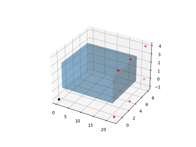
Fig. 13 Mesh with leads as red dots and ground lead as black dot

We will now compute the pseudo-ecg using the recovery formula. In this approach we estimate the extracellular potential using the formula

\[ \phi_b(\mathbf{x}, t) = \frac{1}{4 \pi \sigma_b} \int_{\Omega} \frac{ M_i \nabla V(\tilde{\mathbf{x}}, t) (\tilde{\mathbf{x}} - \mathbf{x})}{\| \tilde{\mathbf{x}} - \mathbf{x} \|^3} \mathrm{d}\tilde{\mathbf{x}} \]

And we compute the pseudo-ECG by subtracting \(\phi_b(\mathbf{x}_p, t) - \phi_b(\mathbf{x}_g, t)\) where \(\mathbf{x}_p\) is the position of the lead and \(\mathbf{x}_g\) is the position of a ground lead.

def voltage_traces():
    for t in time_stamps:
        yield loader.get("ep", "V", t)


fig, ax = plt.subplots()
for point in points:
    ecg = simcardems.postprocess.ecg(
        voltage_traces(),
        sigma_b=1.0,
        point1=point,
        point2=(-10.0, -10.0, -10.0),
    )

    ax.plot(np.array(time_stamps, dtype=float), ecg, label=point)
ax.legend()
fig.savefig(outdir / "ecg.png")

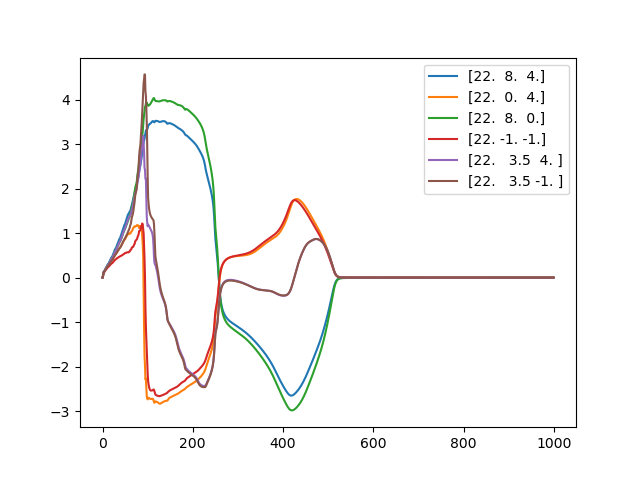
Fig. 14 Pseudo-ECG

Next we use a function for computing the activation map, and indicate that the threshold value should be 0.0. The activation map, will then be a function over the mesh where the value at a given point will be the time it takes for the voltage to first reach 0.0 mV.

activation_map = simcardems.postprocess.activation_map(
    voltage_traces(),
    time_stamps=time_stamps,
    V=loader._functions["ep"]["V"].function_space(),
    threshold=0.0,
)

and compute the activation times for all points through the center of the mesh, from \(x=0\) to \(x=L_x\).

x = np.linspace(0, geo.parameters["lx"], 50)
act = [
    activation_map(xi, geo.parameters["ly"] / 2, geo.parameters["lz"] / 2) for xi in x
]
fig, ax = plt.subplots()
ax.plot(x, act)
ax.set_xlabel("$x$ coordinate")
ax.set_ylabel("Activation time [ms]")
ax.grid()
fig.savefig(outdir / "activation_times.png")

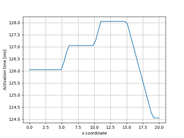
Fig. 15 Activation times through the center of the mesh.