Left ventricular geometry

In this demo we will run the same simple demo but using a ventricular geometry instead. Note that we currently only support a fixed base boundary condition, but plan to add support for more complicated boundary conditions in the future.

Import the necessary libraries

import pprint
from pathlib import Path

import simcardems

# Create configurations with custom output directory
here = Path(__file__).absolute().parent
outdir = here / "results_lv_ellipsoid"

# Specify paths to the geometry that we will use
geometry_path = here / "geometries/lv_ellipsoid.h5"
geometry_schema_path = here / "geometries/lv_ellipsoid.json"

config = simcardems.Config(
    outdir=outdir,
    geometry_path=geometry_path,
    geometry_schema_path=geometry_schema_path,
    T=1000,
    coupling_type="explicit_ORdmm_Land",
    mechanics_solve_strategy="fixed",
    spring=0.01,
)

# Print current configuration
pprint.pprint(config.as_dict())

runner = simcardems.Runner(config)
runner.solve(T=config.T, save_freq=config.save_freq, show_progress_bar=True)

This will create the output directory results_simple_demo with the following output

results_simple_demo
├── results.h5
├── results.json
├── state.h5
├── state.json

The file state.h5 contains the final state which can be used if you want use the final state as a starting point for the next simulation. The file results.h5 contains different traces such as Displacement (\(u\)), active tension (\(T_a\)), voltage (\(V\)) and calcium (\(Ca\)) for each time step. The .json files are used to load load the geometries and, see https://computationalphysiology.github.io/cardiac_geometries/quickstart.html#schema for more info. We can also plot the traces using the postprocess module.

simcardems.postprocess.plot_state_traces(outdir.joinpath("results.h5"))

Here the traces generated by averaging over this domain.

This will create a figure in the output directory called state_traces.png which in this case is shown in Figure 6 we see the resulting state traces, and can also see the instant drop in the active tension (\(T_a\)) at the time of the triggered release.

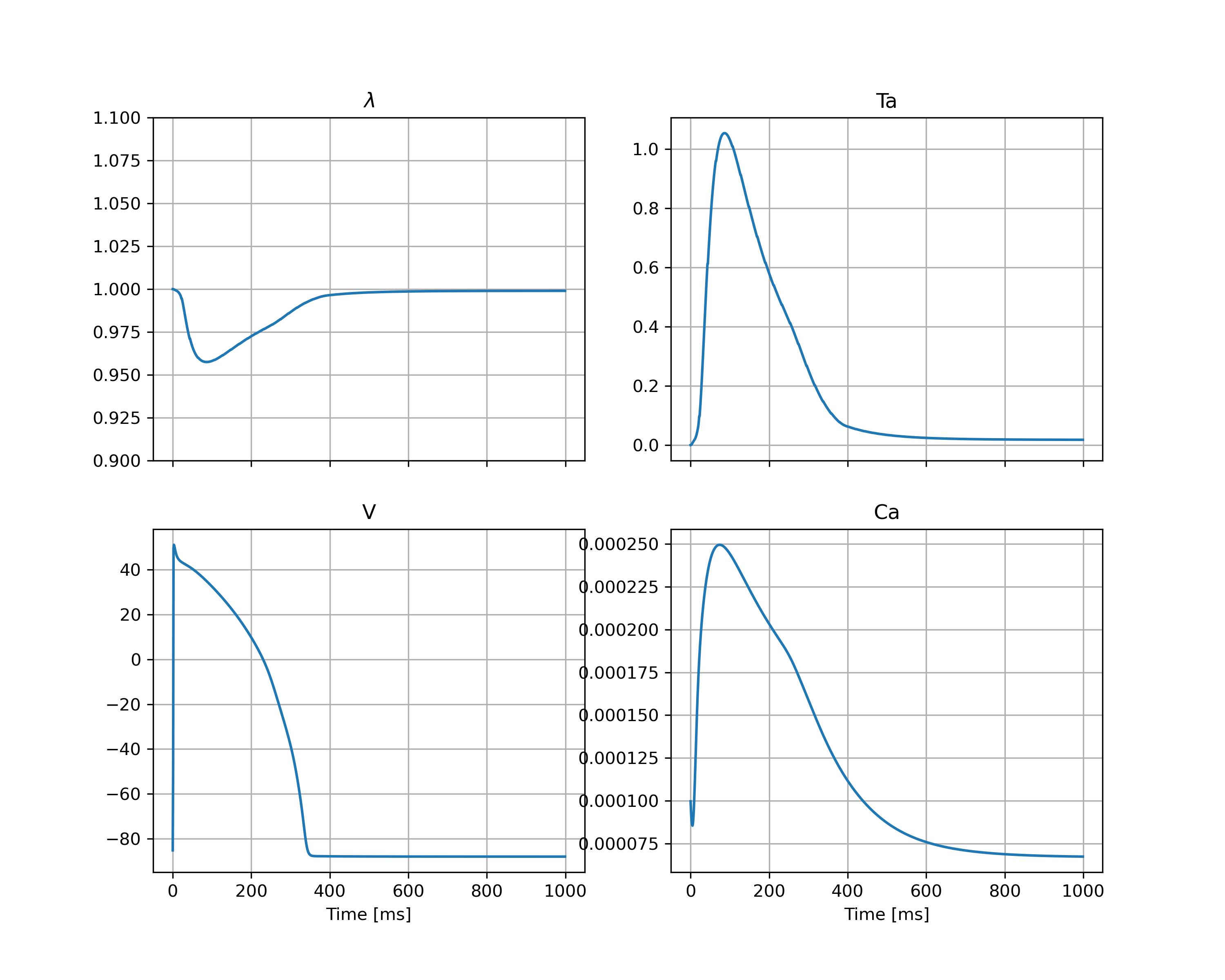
Fig. 6 Traces of the stretch (\(\lambda\)), the active tension (\(T_a\)), the membrane potential (\(V\)) and the intercellular calcium concentration (\(Ca\)) at the center of the geometry.

We can also save the output to xdmf-files that can be viewed in Paraview

simcardems.postprocess.make_xdmffiles(outdir.joinpath("results.h5"), names=["u"])

Displacement (\(u\)), active tension (\(T_a\)), voltage (\(V\)) and calcium (\(Ca\)) visualized using Paraview.