Tracking Values

So far we have only seen how you can track states and intermediates at every node in the mesh. This will quickly use a lot of storage if you are running big simulations. However, for some state variables you might only be interested in tracking the value of some states at a particular node or just the average. For the slab geometry for instance we might want to only track certain variables at the center of the slab, as an average over the entire mesh, or you want to track the full states.

First we will make the necessary imports.

import simcardems
from pathlib import Path
import matplotlib.pyplot as plt

We will use the fully coupled model as the base model, but we will adjust which variables are collected and how they are collected.

The way we specify how to collect a certain variable is through the register_datacollector, so in order to change the way we collect the data we need to override this method. By default, this method will take all the functions that are part of self.assigners and store the full function of each of them. By specifying the argument reduction we can change the way individual variables are stored. By default, the value of this argument is "full" which mean that the full function is stored. Another option that is always available is the value "average" which will store the average value (i.e integrated over the domain and divide by the volume of the domain).

One thing to note is that in order to be able to create xdmf-files you need to store the "full" function.

Different geometries might implement different types of reductions. For the the SlabGeometry we can also evaluate at some prescribed nodes, for example at the center, see https://computationalphysiology.github.io/simcardems/api.html#module-simcardems.value_extractor for all options.

class EMCoupling(simcardems.models.fully_coupled_ORdmm_Land.EMCoupling):
    def register_datacollector(self, collector) -> None:
        for group_name, group in self.assigners.functions.items():
            for func_name, func in group.items():
                reduction = "full" if func_name in ["V", "u"] else "center"
                collector.register(
                    group=group_name,
                    name=func_name,
                    f=func,
                    reduction=reduction,
                )

        collector.register(
            "mechanics",
            "lambda_center",
            self.lmbda_mech,
            reduction="center",
        )
        collector.register("mechanics", "lambda", self.lmbda_mech, reduction="average")
        collector.register(
            "mechanics",
            "Ta",
            self.mech_solver.material.active.Ta_current,
            reduction="average",
        )
        self.mech_solver.solver.register_datacollector(collector)

In this example we will store the full function (i.e value at each node) of V, u. For the rest of the variables we will either pick an average value or the value at the center of the slab. Notice also that we store both the average lambda and the value of lambda that is evaluated at the center of the slab.

We are now ready to run the model. First, we need to load the slab geometry

geo = simcardems.geometry.load_geometry(mesh_path="geometries/slab.h5")

Now, we need to create the custom coupling object. Note however that the CellModel and the ActiveModel remains the same

coupling = simcardems.models.em_model.setup_EM_model(
    cls_EMCoupling=EMCoupling,
    cls_CellModel=simcardems.models.fully_coupled_ORdmm_Land.CellModel,
    cls_ActiveModel=simcardems.models.fully_coupled_ORdmm_Land.ActiveModel,
    geometry=geo,
)

We also need to create the configuration, and we pass in the output directory and the coupling_type.

outdir = Path("results_tracking_values")
config = simcardems.Config(
    outdir=outdir,
    coupling_type=coupling.coupling_type,
)
# Now we create a runner for running the simulation

runner = simcardems.Runner.from_models(coupling=coupling, config=config)

And then we run a simulation for 1000 milliseconds

runner.solve(1000)

When the simulation is done we can load the results from the output directory using simcardems.DataLoader

loader = simcardems.DataLoader(outdir / "results.h5")

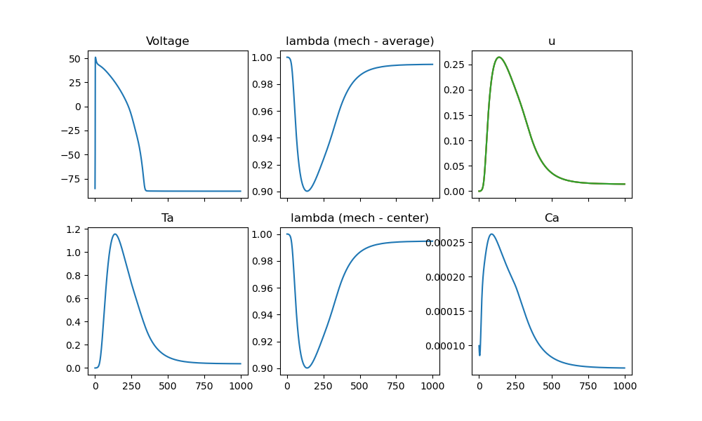
We can extract the traces from the loader. Here you should also pass a value for the reduction, but this will only be applied if the trace you want to extract is a function.

values = simcardems.postprocess.extract_traces(loader, reduction="average")

fig, ax = plt.subplots(2, 3, sharex=True, figsize=(10, 6))
ax[0, 0].plot(values["time"], values["ep"]["V"])
ax[0, 0].set_title("Voltage")

ax[1, 0].plot(values["time"], values["mechanics"]["Ta"])
ax[1, 0].set_title("Ta")

ax[0, 1].plot(values["time"], values["mechanics"]["lambda"])
ax[0, 1].set_title("lambda (mech - average)")

ax[1, 1].plot(values["time"], values["mechanics"]["lambda_center"])
ax[1, 1].set_title("lambda (mech - center)")

ax[0, 2].plot(values["time"], values["mechanics"]["u"])
ax[0, 2].set_title("u")

ax[1, 2].plot(values["time"], values["ep"]["Ca"])
ax[1, 2].set_title("Ca")

fig.savefig(outdir / "tracking_values.png")

Fig. 9 Showing the Output of the tracked values

You can also create XDMF-files, and the only the variables that are stored as full functions can be used for creating XDMF-files. Here we also specify that we only want to create an XDMF-file for u.

simcardems.postprocess.make_xdmffiles(outdir.joinpath("results.h5"), names=["u"])