Simple demo

In this demo we show the most simple usage of the simcardems library using the python API.

Import the necessary libraries

from pathlib import Path
import simcardems

# First we specifcy the path to the output directory where we want to store the results
here = Path(__file__).absolute().parent
outdir = here / "results_simple_demo"

Next we specify paths to the geometry that we will use, and we will use the slab geometry that already exist in the demo folder.

geometry_path = here / "geometries/slab.h5"
geometry_schema_path = here / "geometries/slab.json"
# The geometry contains a path to the mesh itself (togther with other functions such as meshfunctions and fibers), and a path to a schema which describes what information that can be found in the geometry file. Please see https://computationalphysiology.github.io/cardiac_geometries/ for more info about the geometries
#
# Next we create the configuration. Here we specify the the output directory, the path to the geometry, how long we want to simulate and the coupling type. We use the `fulle_coupled_ORdmm_Land` coupling type which contains the stronlgy coupled O'Hara-Rudy model coupled to the Land model. The other options here are `explicit_ORdmm_Land` where the coupling is explicit and `pureEP_ORdmm_Land` which will run a pure EP simulation without mechanics.

config = simcardems.Config(
    outdir=outdir,
    geometry_path=geometry_path,
    geometry_schema_path=geometry_schema_path,
    loglevel=10,
    coupling_type="fully_coupled_ORdmm_Land",
    T=20,
)

To see all different configuration options you can visit https://computationalphysiology.github.io/simcardems/api.html#module-simcardems.config

Next we create a runner for running the simulation, and we also specify how often we want to save the results

runner = simcardems.Runner(config)
runner.solve(T=config.T, save_freq=config.save_freq, show_progress_bar=True)

Once the simulation is done the output directory results_simple_demo will contain the following files

results_simple_demo
├── results.h5
├── state.h5

The file state.h5 contains the final state which can be used if you want use the final state as a starting point for the next simulation. The file results.h5 contains output of different state variables for every time point.

We can now plot the state traces, where we also specify that we want the trace from the center of the slab

simcardems.postprocess.plot_state_traces(outdir.joinpath("results.h5"), "center")

This will create a figure in the output directory called state_traces_center.png which in this case is shown in Figure 1 we see the resulting state traces, and can also see the instant drop in the active tension (\(T_a\)) at the time of the triggered release.

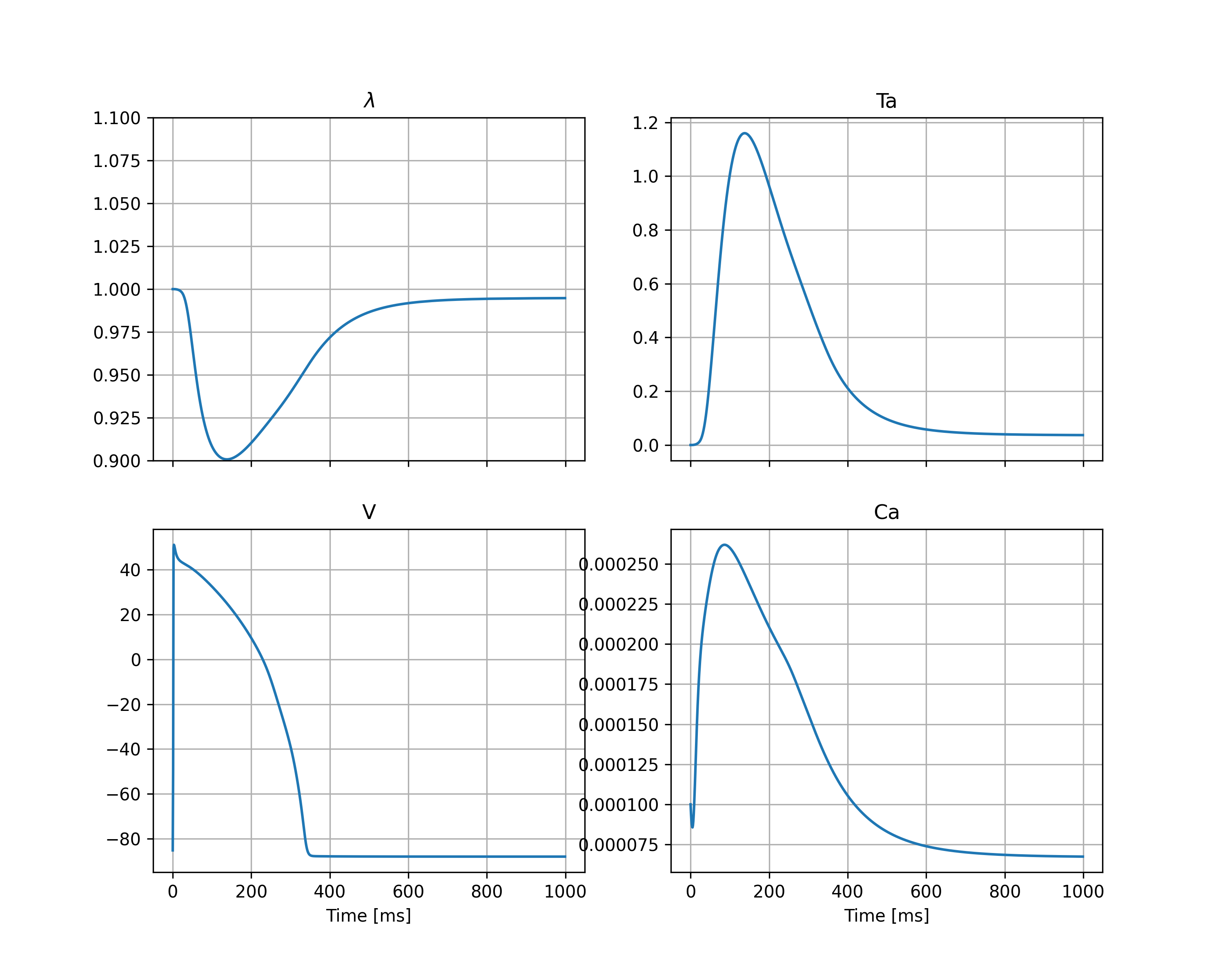
Fig. 1 Traces of the stretch (\(\lambda\)), the active tension (\(T_a\)), the membrane potential (\(V\)) and the intercellular calcium concentration (\(Ca\)) at the center of the geometry.

We can also save the output to xdmf-files that can be viewed in Paraview

simcardems.postprocess.make_xdmffiles(outdir.joinpath(“results.h5”))

The xdmf files are can be opened in Paraview to visualize the different variables such as in Figure 2.

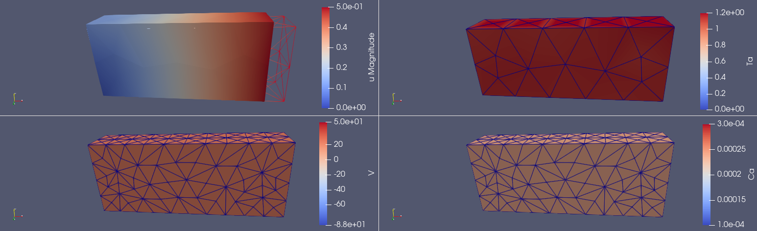
Fig. 2 Displacement (\(u\)), active tension (\(T_a\)), voltage (\(V\)) and calcium (\(Ca\)) visualized for a specific time point in Paraview.